


Services on Demand
Journal
Article
 text in
  English (pdf)
 Article in xml format
 Article references
 Send this article by e-mail
Indicators
-
 Cited by SciELO
 -
 Access statistics
Related links
-
 Similars in
SciELO
Similars in
SciELO
Share

 Permalink
Agrociencia
On-line version ISSN 2521-9766Print version ISSN 1405-3195
Agrociencia vol.52 n.6 Texcoco Aug./Sep. 2018
Water-Soil-Climate
Comparative analysis of prescribed burns applied to tropical oak woodlands
1División de Ciencias Forestales, Universidad Autónoma Chapingo. km. 38.5 carretera México-Texcoco. 56230. Chapingo, Estado de México México. normonjaras@gmail.com
2Escuela Técnica Superior de Ingeniería Agraria, Universidad de Lerida. Avenida Rovira Roure 191, 25198 Lerida, España. jorgepulidoluna@gmail.com
3Biomasa, A. C. Segunda Norte no. 62, entre Tercera y Cuarta Oriente, Barrio Matzumóm. 30470. Villaflores, Chiapas,México. pmtz29@hotmail.com
4Universidad de Ciencias y Artes de Chiapas, Sur Poniente 1460, Colonia Centro. 29000. Tuxtla Gutiérrez, Chiapas, México. pmtz_19@hotmail.com
Forest fires and agricultural burns contribute to global climate change, and the latter is a tool that reduces CO2 emissions. The objective of this study was to evaluate the consumption of surface fuels, fire behavior, and emissions in prescribed burns. The hypothesis was that fires affect more fuels and produce more emissions than prescribed burns. Prescribed burns were applied in six randomly-established experimental plots in a tropical oak woodland in Chiapas, Mexico: three heading and three backing fires. Measurements and estimates included: initial and residual fuel loads, consumption factors, and CO2 emissions. Wind speed and direction, temperature and relative humidity, fire spread rate, and flame length were recorded during the burns. In a forest fire, the flame length and the residual fuel load were determined. The t- and the Wilcoxon (under lack of normality) tests were applied. In the heading and backing fires, there were significant differences in the fire spread rate (3.63 and 0.59 m min-1), but there were none in the flame length (0.91 and 0.72 m). The flame length of fires reached 1.94 m, but burns had different results. The total fuel loads in backing and heading fires were 28.393 and 35.512 t ha-1, without differences between them; the consumption factors for backing and headingfires and forest fire reached 92.7, 87.5, and 97.2 %, without showing any difference; however, the forest fire affected aerial fuels. The CO2 emissions reached 44.53, 51.14, and 53.78 t CO2 ha-1. The prescribed burns help to reduce emissions, because their intensity and severity are lower than those of forest fires. Consequently, since burns affect a smaller surface, they help to prevent fires and to reduce emissions.
Keywords: CO2; climate change; greenhouse effect; fire; fire management
Los incendios forestales y las quemas agropecuarias contribuyen al cambio climático global y una herramienta para reducir emisiones de CO2 es el fuego prescrito. El objetivo de este estudio fue evaluar consumo de combustibles superficiales, comportamiento del fuego y emisiones en quemas prescritas. La hipótesis fue que los incendios afectan más combustibles y producen mayores emisiones que las quemas. En seis parcelas experimentales de un encinar tropical de Chiapas, México, establecidas al azar, se aplicaron quemas prescritas: tres a favor de viento y pendiente y tres en contra. Las mediciones y estimaciones incluyeron: las cargas iniciales y residuales de combustibles, factores de consumo y emisiones de CO2. Durante las quemas se registraron dirección y velocidad del viento, temperatura y humedad relativa, velocidad de propagación del fuego y longitud de llama. En un área bajo afectación por incendio, se determinó la longitud de la llama y la carga residual de combustibles. La prueba de “t” y la de Wilcoxon se aplicaron cuando hubo falta de normalidad. En las quemas a favor y en contra, las diferencias en velocidad de propagación (3.63 y 0.59 m min-1) fueron significativas, pero en la longitud de llama (0.91 y 0.72 m) no. En el incendio, esta última alcanzó 1.94 m, con diferencias con respecto a las quemas. Las cargas totales de combustibles en quemas en contra y a favor fueron 28.393 y 35.512 t ha-1, sin diferencias entre sí; los factores de consumo para quema en contra, a favor e incendio, alcanzaron 92.7, 87.5 y 97.2 %, sin diferencias, pero con afectación de combustibles aéreos por el incendio. Las emisiones de CO2 alcanzaron 44.53, 51.14 y 53.78 t CO2 ha-1. Debido a su intensidad y severidad menores que en los incendios, por prevenirlos y afectar una superficie menor, las quemas prescritas son útiles para reducir emisiones.
Palabras clave: CO2; cambio climático; efecto invernadero; fuego; manejo del fuego
Introduction
Mexico is the richest country in Quercus species, with 157 of them. The majority can be found in temperate and semi-arid zones, as well as in tropical zones (Zavala, 2007). Most of these oaks are adapted to fire, but some species in the tropical and subtropical regions of the country -particularly in the tropical cloud forest- are sensitive to this factor (Rodríguez and Myers, 2010). Thirty-one species of Quercus can be found in Chiapas (Zavala, 2002). These species have adapted to fire in several ways: small seeds -which do not require a high level of humidity to establish themselves, in comparison with large seed species-; initial successional stages -since they colonize sites disturbed by agents such as fire-; thick bark -which isolates the vascular cambium from high temperatures-, and the capacity to resprout -which allows them to recover from damage (Rodríguez and Myers, 2010; Rodríguez, 2014; López et al., 2015). Fire also has successional implications for oaks. For example, oak woodlands in eastern USA are maintained by fire, to the detriment of Carya, a more mesophytic genus that is less tolerant to this factor (Dickinson et al., 2016).
Fire is an ecological factor in many ecosystems of the planet (Whelan, 1997) and of Mexico (Rodríguez, 2014); however, the anthropogenic alteration of fire regimes has resulted in tropical ecosystems representing around half of the area affected by fires in the world (Cochrane, 2009). As a result, in the 1997-2009 period, fires represented an average annual emission of 2 Pg C year-1 in tropical ecosystems (van der Werf et al., 2010).
Due to the greenhouse effect, the USA and Canada begin to experience longer fire seasons, more lightning fires, increasingly severe droughts, and more areas affected by forest fires of great intensity and severity (Ryan, 2000). Climate change can increase the negative effects of fires in several ecosystems, increase greenhouse gas emissions, and hinder fire control, making it more expensive and dangerous. In addition, the extreme El Niño event in 2014-2016 generated high temperatures and drought, increased the impact of severe fires in Asia, and reduced carbon capture in the Amazon rainforest. Likewise, the temperature in Africa increased, but the precipitation remained largely the same, resulting in a higher release of CO2. These three processes issued 3 (10)9 t C in 2014-2016, equivalent to 20 % of the emissions caused by the burning of fossil fuels and cement manufacturing (Popkin, 2017).
Global climate change alters the factors that control fire, including: temperature, precipitation, humidity, wind, ignition, biomass, dead organic matter, composition and structure of vegetation, and soil humidity. Such changes threaten the proper functioning of ecosystems and the provision of ecosystem services (IPCC, 2001; Hassan and Ash, 2005; Shlisky et al., 2007).
The prescribed burns have different uses, such as: decreasing fire danger; reducing forest exploitation waste; favoring regeneration or preparing the area for reforestation; improving wildlife habitat; promoting the use of forage for grazing; improving aesthetics and access; and controlling invasive species (Wade and Lunsford, 1989; Holmes et al., 2011). In addition, since their species are adapted to fire, they can help to reduce forest fires -and the resulting contribution to the greenhouse effect- in ecosystems maintained by fire (such as pine and oak, including the tropical ones).
Researches about forest fuel loads, fire behavior, and greenhouse gas emissions serve various crucial purposes, such as the estimation of fire danger, the definition of forest fuel models and their dynamics, and the modeling of fire behavior and its effects, as well as the modeling of greenhouse gas emissions (both during forest fires and prescribed burns).
Therefore, this study had the following objectives: 1) to determine the fuel load in a tropical oak woodland; 2) to study the behavior of prescribed burns (heading and backing fires; and slope); 3) to determine fuel consumption factors; 4) to estimate the CO2 emission; and 5) to estimate the immediate severity of the fire in each treatment. The hypothesis was that fires affect more fuels and generate higher emissions than prescribed burns.
Materials and Methods
Field sampling
Initial sampling, residual fuel sampling, and fuel harvesting
In February 2016, the study area was selected: a tropical oak woodland in the rural community of Villahermosa, Municipality of Villaflores, Chiapas (Figure 1). The zone has a sub-humid warm climate (Aw2), with 22 to 24 °C isotherms and 1200- to 1500-mm isohyets. The terrain is uneven, mostly dominated by sedimentary and volcano-sedimentary rocks; it belongs to the regosol soil group and the dominant vegetation is the pine-oak association (Ecosur, 2018). Stands of oaks can be found where the study was carried out and the most common species are Quercus peduncularis Née, Q. skinneri Benth. and Q. magnoliifolia Née. Six 0.5-ha plots were established. The measurement of forest fuels involved the establishment of triangular sampling sites in the center of each plot, with stakes marking the vertices (Figure 2). The triangular design had the purpose of concentrating fuel sampling as much as possible around the sampling lines utilized to measure fire behavior. For woody fuels, the Brown’s Planar Intercept Method (1974) was used, and for leaf litter, fermentation layer, forbs, grasses, shrubs, and regeneration, the measuring and harvest method was used. The 12-m sides of the sampling triangle -and the base following the contour line- were used as sampling lines for woody fuels. The slope of each of the triangle’s sampling lines was measured with a Suunto© clinometer. Starting from each vertex and working in clockwise direction, 2-, 4-, and 12-m long overlapping lines were established. The 2-m lines were used to record the number of fuel intersections with 1 h of time lag (TR) (<0.6 cm diameter), as well as for those with 10 h of TR (0.6 to 2.5 cm). The 4-m lines were used to record the quantity of fuel intersections with 100 h of TR (2.6 to 7.5 cm). The 12-m line was used to record the intersections with materials with 1000 h of TR, both sound and rotten (˃7.5 cm). In this last case, the diameter of each piece was also recorded. For each TR, 12 specimens of woody materials were collected in order to determine their specific gravity in the laboratory.
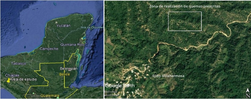
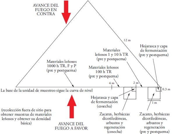
Figure 2 Cluster sampling for forest fuels. Site 1 is shown in detail, but sites 2 and 3 (the other sides of the triangle) had the same components and were also sampled.
Next to each vertex square sampling sites were established on the outside of the triangle, without trampling on the area. The sites had the following dimensions (fuel type indicated in parentheses): 0.3X0.3 m, metal frame (leaf litter and fermentation layer); 1X1 m, rigid plastic frame (PVC) (forbs and grasses), and 4X4 m, with measuring tape (shrubs and regeneration). The leaf litter and fermentation layer coverage (%) was estimated visually, while its layer depth was measured in four points with a measuring tape. The coverage of the remaining fuel was estimated (%) and six height measurements were made. Additionally, all the fuels were sampled again 2 m ahead of these sites and on each side of the triangle. In these last sitios, after they were measured, the materials were harvested, put in brown paper bags, labeled, and placed in plastic bags. As it is explained below, this sampling and harvest were carried out to determine dry weight.
In order to sample the different fuels, 11 sampling sites were established per side, resulting in 33 sites per triangle, and 198 sites for the six triangles. The sampling aimed at harvesting and obtaining dry weights included 6 sites per side, 18 sites per triangle, and 108 sites in total. The three fuel samplings (initial, harvest and residual) involved 504 sampling sites.
Prescribed burns and sampling of meteorological variables
As part of our experiment, six prescribed burns were carried out in March 2016. Each 0.5 ha plot where fuel was sampled was subject to a burn. Three of them were carried out as heading fires, and three were carried out as backing fires. The authors oversaw the prescription. Authorization for research purposes was requested from and granted by the local CONAFOR office, in accordance with the official Mexican Fire Use Standard NOM-015 (SEMARNAT). Two crews (one community and one municipal), made up by 10 elements each, carried out the prescribed burns. One crew was in charge of the burns, and the other was ready to spring into action, in case the fire went out of control. The burns were planned and directed by the authors and José Domingo Cruz López (CONANP). Security measures were implemented, in case the burns went out of hand and to protect the staff; those measures were based on the Incident Management System. In addition, three community crews oversaw the measurements; each one had three members, who were guided and supervised by the authors. These brigades had been previously trained to perform and record part of the observations that were necessary for our research.
The prescribed burn plots were representative of the conditions present in the area and they were randomly distributed in a small basin, with openings to the N, N-NE, NE, E and SE cardinal points. The slopes of the terrain had a 50 to 90 % interval (average: 73 %).
The weather was recorded during the prescribed burns, using a portable meteorological kit (Forestry Supplyers, Inc.©). The kit includes: an anemometer (to measure the wind speed); a compass (to determine its direction); a sling psychrometer (to obtain dry and wet bulb temperatures); and a nomogram (ruler) (to estimate the relative humidity). The weather was observed five times during each prescribed burn (30 times in total).
The fire behavior sampling line was placed in the center of the prescribed burn plot -as well as at the center of the fuel sampling triangle-, perpendicular to its base. Dry and wet bulb temperatures, as well as relative humidity, were recorded when the fire touched the first sampling stake. The direction and speed of the wind was obtained every time the fire reached each stake.
Fire behavior
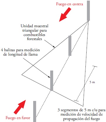
Flame length (LL) and fire spread rate (VP) were measured as fire behavior variables. For this purpose, a 2 m long stake was fixed in the center of the base of the triangle to measure forest fuels, while red and white bands were painted every 0.2 m. Three stakes were placed upwards the slope and one downwards, 5 m apart from each other. The flame length was measured when it reached the stake. The VP was estimated based on the time that the fire required to cross each 5 m section. Fire behavior was measured in 18 sampling sites (Figure 3).
Immediate fire severity in the trees
In each burn plot, a 1000 m2 site was settled for ≥2 m high trees. The genus, height, and diameter at breast height of the trees were documented. Crown scorch (CHC) and height of fire scar on trunk (CT) were recorded as fire severity variables. In total, six of this type of site were placed.
Forest fire sampling
A forest fire began in a nearby area, at the same time that the forest fuel sampling was carried out. The fire affected 10 ha, before it was controlled by municipal and community brigades. The research team had the opportunity to carry out six LL measurements, as well as three residual fuel and severity in the trees measurements, which were useful for this work. The initial fuel load was considered as the average of the heading and backing fires, and three residual fuel sampling sites were settled there. Three severity sampling sites were also placed in this area.
Laboratory and desk research
Initial and residual loads of forest fuels
The samples of harvested fuel were taken to the Laboratorio de Nutrición Animal of the Universidad Autónoma de Chiapas, where they were placed in drying ovens at 70 °C and weighed until they reached constant weight. The dry weight of each sample was connected with the imaginary rectangular prism obtained in the field, product of the multiplication of coverage (as a proportion of one) by the average height or depth, depending on the type of fuel. Based on the resulting averages, the initial and residual loads of the prescribed burnings were estimated for the fuels sampled in the field. Finally, the loads were extrapolated to t ha-1.
The models used for woodfuels require information about their specific gravity. This information was gathered from samples of this type of fuel that were collected from the forest floor. According to Van Wagner (1968), Brown (1974), and Morfín et al. (2012), the models used to obtain the loads (C) of woody materials from 1 to 100 h TR (1) and for 1000 h TR (both sound and rotten) were:
where k=1.234, GE=specific gravity, DCP=quadratic mean diameter, f=frequency of intersections, c=factor for the slope of the sampling line, N=number of sampling lines, L=length of the sampling line, ΣDC=summation of quadratic diameters.
Estimation of emissions
The calculation of the fuel load consumed by fire (Cc), the consumption factor (F), and the emissions (E) (IPCC, 2001), involved the following models in each sampling site:
where C=initial fuel load, Cr=residual fuel load, S=surface, and Fe=emission factor.
Fe=1.703 t CO2 ha-1, the same than for prescribed burns in pine-oak forests in southeastern USA, according to several authors and quoted by Urbanski (2013).
Statistical analysis
The variables studied were compared between heading and backing fire treatments, using the Student’s t-test (p≤0.05), with a variance inequality test. Likewise, the graphic method was used to establish normality. If normality was lacking, the Wilcoxon test (its exact value) was used. For all analyses, the Proc ttest and Proc nPar1way procedures of the SAS v. 9.4 statistical software for microcomputers were used.
RESULTS AND DISCUSSION
Weather
During the prescribed heading fires, the means and their standard deviation (in parentheses) of wind speed, temperature, and relative humidity were 4.77 km h-1 (2.85), 27.4 °C (5.61), and 60.2 % (19.83), respectively. Meanwhile, during the backing fires, the averages reached 3.97 km h-1 (2.69), 31.2 °C (2.05), and 52 % (29.36), respectively. In the case of the above-mentioned variables, the inequality of variances test had the following p-values: 0.8275, 0.0006, and 0.1543. As a result, only temperature showed inequality of variances. Only this last variable showed significant differences between both treatments (p=0.027); wind speed (p=0.445) and relative humidity (p=0.338) did not show significant differences. The three atmospheric variables under consideration lacked normality; therefore, the p of the exact value of the Wilcoxon test was used (0.523, 0.169, and 0.406). In other words, there were no differences between the medians of the variables of the applied treatments. However, although there were no differences in the wind speed, the wind blew against the fire in backing fires, so the test was also applied with negative wind speed values for this variable. In this case, the mean and its standard deviation was -3.97 km h-1 (2.69), there was no inequality of variances (p=0.827), and there were significant differences with the t-test (p≤0.001). There was no normality and the Wilcoxon test showed differences between medians (p≤0.001). In both burn methods, the means of the weather parameters were below the limits that Wade and Lunsford (1989) established as an adequate prescription (up to 5-16 km h-1 wind speed, 30 to 55 % relative humidity). That is not the case of temperature (18-27 °C), although the said authors mention that it recorded in cold temperate climate or temperate climate zones.
Fire behavior
In the heading fire, the VP variable reached a mean and standard deviation (in parentheses) equal to 3.63 m min-1 (3.41), while for the backing fire, it was 0.59 m min-1 (0.26). There was inequality of variances (p≤0.001) and significant differences for this variable with the t-test (p=0.028). There was no normality, and -with the Wilcoxon test- there were differences between medians (p=0.003). Due to safety and accessibility issues, no fire VP measurements were obtained, but they were estimated at ˃30 m min-1. LL reached 0.91 (0.28) and 0.72 m (0.30), in both heading and backing fires. The variances were similar (p=0.837) and there were no differences between both treatments (p=0.188). In this case, there was no normality and the Wilcoxon test produced no significant results (p=0.129).
In the forest fire, LL reached a mean of 1.94 m (1.06). Variances were unequal (p=0.016) and the t-test showed no differences (p=0.063). There was no normality either and the Wilcoxon test showed significant differences between the medians (p=0.033).
The figures for weather and fire behavior matched those of other researches. Experimental prescribed burns were carried out in a tropical oak woodland of Q. magnoliifolia in Guerrero. The weather had the following characteristics: temperature between 25 and 28 °C, with 33 to 25 % relative humidity, wind speed of 7 to 8 km h-1, and gusts up to 25 km h-1. LLs ranged from 0.5 to 3 m and there was a direct logarithmic relationship in which LL is a function of wind speed (López et al., 2015). In pine-oak forests in Chihuahua where Pinus duranguensis Martínez and Q. sideroxyla A. J. A. Bonpland can be found, prescribed burns -carried out with a relative humidity around 60 %, winds of 2 to 6.1 km h-1, and temperatures of 1.5 to 14.5 °C- showed LL of 1 to 6 m, and PV of 0.8 up to 5 m min-1 (Flores et al., 2010).
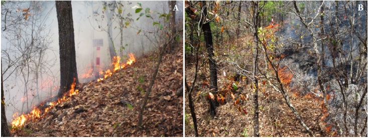
The largest VP and LL in heading fires are known. The wind provides oxygen to the combustion, tilts the convective column and the flame, and brings them closer to the unburned materials, drying them and making them available quicker; in addition, it generates flying sparks. As the fire rages on, the fuels found uphill dry quicker than those found downhill, because they are closer to the convective column and the radiation and the fire in the front line is more intense; this situation accelerates the combustion and VP (Scott et al., 2014). The few differences between the heading and backing fires are based on the fact that (for safety purposes) both were carried out under moderate weather conditions (Figure 4). Regarding the topography, Franklin et al. (1997) established that the slope is of particular importance for the intensity of the fire in leaf litter fuel beds and the fermentation layer of North American oak woodlands.
Initial and residual loads of forest fuels
In this case, the following variables were compared for the two types of burns: the partial loads for each type of forest fuel, the sum of woody fuels, and the total load. Likewise, the residual load, the load consumed, the proportion of load consumed, and the consumption factor were compared. Most of the variables showed a lack of normality. The Wilcoxon test showed that there were only differences in medians between the backing and the heading fires for the following elements: residual load of leaf litter, consumption factor of leaf litter, initial grass load, and grass consumption. Comparing total load, residual load, total consumed load, and their consumption factor, there were no differences between any of these variables for these types of burn. This analysis is shown in Table 1 (leaf litter and fermentation layer), Table 2 (grasses, forbs, shrubs, and regeneration), Table 3 (woody materials with TR 1, 10, and 100 h), Table 4 (sound and rotten woody materials with TR 1000 h), Table 5 (total load of woody fuels), and Table 6 (total load of forest fuels). No differences were found between forest fire and heading fires, and then between forest fire and backing fires, when comparing the following variables: total and residual load, consumption, and consumption factor.
Table 1 Average loads (t ha-1) and statistical analysis results for leaf litter and fermentation layer.
| Var. |
|
|
Des. σ2 | p | p (t) | Nor. | p (Wil.) |
|---|---|---|---|---|---|---|---|
| CH | 2.6702 (2.1535) | 4.8780 (2.3462) | no | 0.8143 | 0.0540 | sí | ns |
| CrH | 0.0043 (0.0130) | 0.1161 (0.2109) | sí | <0.0001 | 0.1510 | no | 0.0294* |
| CcH | 2.6659 (2.1582) | 4.7619 (2.3992) | no | 0.7718 | 0.0691 | sí | ns |
| FH | 99.29 (2.13) | 95.18 (11.55) | sí | <0.0001 | 0.3227 | no | 0.0430* |
| CCF | 10.7007 (17.2742) | 13.9840 (25.6416) | no | 0.2847 | 0.7547 | no | ns |
| CrCF | 0.1202 (0.2795) | 3.8706 (9.3175) | sí | <0.0001 | 0.2619 | no | ns |
| CcCF | 10.5865 (17.3202) | 10.1134 (18.8131) | no | 0.8208 | 0.9750 | no | ns |
| FCF | 92.27 (19.81) | 92.36 (17.08) | no | 0.8076 | 0.9932 | no | no |
Table 2 Average loads (t ha-1) and statistical analysis results for live surface fuels.
| Var. |
|
|
Des. σ2 | p | p (t) | Nor. | p (Wil.) |
|---|---|---|---|---|---|---|---|
| CZ | 0.9397 (1.957) | 0 (0) sí | sí | <0.001 | 0.188 | no | 0.009* |
| CrZ | 0 (0) | 0 (0) | - | - | - | - | - |
| CcZ | 0.9737 (1.957) | 0 (0) sí | sí | <0.001 | 0.188 | no | 0.009* |
| FZ | 100 (0) | - | - | - | - | - | - |
| CD | 0.440 (0.567) | 0.089 (0.106) | sí | <0.001 | 0.103 | no | ns |
| CrD | 0 (0) | 0 (0) | - | - | - | - | - |
| CcD | 0.4405(0.567) | 0.089 (0.106) | sí | <0.0001 | 0.103 | no | ns |
| FD | 100 (0) | 100 (0) | - | - | - | - | - |
| CA | 1.3658 (2.720) | 1.1148 (2.902) | no | 0.860 | 0.852 | no | ns |
| CrA | 0 (0) | 0.5370 (1.719) | sí | <0.001 | 0.342 | no | ns |
| CcA | 1.3658 (2.720) | 0.5417 (1.202) | sí | 0.033 | 0.423 | no | ns |
| FA | 100 (0) | 80.50 (33.78) | sí | <0.001 | 0.423 | no | ns |
| CR | 0.1375 (0.245) | 0.2187 (0.445) | no | 0.1125 | 0.638 | no | ns |
| CrR | 0 (0) | 0.0117 (0.035) | sí | <0.0001 | 0.347 | no | ns |
| CcR | 0.1375 (0.245) | 0.2070 (0.414) | no | 0.161 | 0.671 | no | ns |
| FR | 100 (0) | 98.35 (3.69) | sí | <0.0001 | 0.374 | no | ns |
CZ=initial grass load; CrZ=residual grass load; CcZ=grass consumption; FZ=grass consumption factor; CD=initial forb load; CrD=residual forb load; CcD=forb consumption; FD=forb consumption factor; CA=initial shrub load; CrA=residual shrub load; CcA=shrub consumption; FA=shrub consumption factor; C=initial regeneration load; CrR=residual regeneration load; CcR=regeneration consumption; FR=regeneration consumption factor.
Table 3 Average loads (t ha-1) and statistical analysis results for thin and medium woody materials.
| Var. |
|
|
Des. σ2 | p | p (t) | Nor. | p (Wil.) |
|---|---|---|---|---|---|---|---|
| C1 | 0.1181 (0.161) | 0.3157 (0.278) | no | 0.504 | 0.348 | no | ns |
| Cr1 | 0.0183 (0.021) | 0.059 (0.085) | no | 0.119 | 0.468 | sí | ns |
| Cc1 | 0.099 (0.140) | 0.257 (0.199) | no | 0.666 | 0.322 | sí | ns |
| F1 | 80.59 (7.90) | 85.51 (12.89) | no | 0.795 | 0.326 | sí | ns |
| C10 | 1.5202 (1.673) | 3.0894 (2.007) | no | 0.820 | 0.357 | no | ns |
| Cr10 | 0.1163 (0.201) | 0.8498 (0.337) | no | 0.527 | 0.032 | no | ns |
| Cc10 | 1.4039 (1.488) | 2.2369 (1.816) | no | 0.804 | 0.571 | no | ns |
| F10 | 94.73 (7.45) | 68.33 (16.07) | no | 0.623 | 0.127 | no | ns |
| C100 | 1.8034 (3.1236) | 2.579 (4.467) | no | 0.6569 | 0.817 | no | ns |
| Cr100 | 0 (0) | 0 (0) | - | - | - | - | - |
| Cc100 | 1.8034 (3.1236) | 2.579 (4.467) | no | 0.657 | 0.817 | no | ns |
| F100 | 100 (-) | 100 (-) | - | - | - | - | - |
C1=initial load of woody materials (1 h TR); Cr1=residual load of woody materials (1 h TR); Cc1=consumption of woody materials (1 h TR); F1=consumption factor of woody materials (1 h TR); C10=initial load of woody materials (10 h TR); Cr10=residual load of woody materials (10 h TR); Cc10=consumption of woody materials (10 h TR); F10=consumption factor of woody materials (10 h TR); C100=initial load of woody materials (100 h TR); Cr100=residual load of woody materials (100 h TR); Cc100=consumption of woody materials (100 h TR); F100=consumption factor of woody materials (100 h TR).
Table 4 Average loads (t ha-1) and statistical analysis results for thick woody materials (with 1000 h TR).
| Var. |
|
|
Des. σ2 | p | p (t) | Nor. | p (Wil.) |
|---|---|---|---|---|---|---|---|
| C1000f | 6.673 (6.089) | 9.243 (16.01) | no | 0.2527 | 0.808 | no | ns |
| Cr1000f | 1.988 (3.443) | 0 (0) | sí | <0.001 | 0.423 | no | ns |
| Cc1000f | 4.68 (6.36) | 9.24 (16.01) | no | 0.273 | 0.670 | no | ns |
| F1000f | 63.16 (52.09) | 100 (-) | - | - | - | - | - |
| C1000p | 2.023 (3.505) | 0 (0) | sí | <0.001 | 0.423 | no | ns |
| Cr1000p | 0 (0) | 0 (0) | - | - | - | - | - |
| Cc1000p | 2.023 (3.505) | 0 (0) | sí | <0.001 | 0.423 | no | ns |
| F1000p | 100 (-) | - | - | - | - | - | - |
C1000f=initial load of sound materials; Cr1000f=residual load of sound materials; Cc1000f=consumption of souond materials; F1000f=consumption factor of sound materials; C1000p=initial load of rotten materials; Cr1000p=residual load of rotten materials; Cc1000p=consumption of rotten materials; F1000p=consumption factor of rotten materials.
Table 5 Average loads (t ha-1) and statistical analysis results for the total woodfuel load.
| Var. |
|
|
Des. σ2 | p | p (t) | Nor. | p (Wil.) |
|---|---|---|---|---|---|---|---|
| CLto | 12.139 (5.261) | 15.227 (22.30) | no | 0.1054 | 0.827 | no | ns |
| CrLto | 2.122 (3.628) | 0.9086 (0.255) | sí | 0.0098 | 0.621 | no | ns |
| CcLto | 18.016 (2.713) | 14.319 (22.138) | sí | 0.0296 | 0.769 | no | ns |
| FLto | 87.73 (20.65) | 75.69 (21.33) | no | 0.9676 | 0.521 | no | ns |
CLto=initial woody fuel load; CrLto=residual woody fuel load; CcLto=woody fuel consumption; FLto=woody fuel consumption factor.
Table 6 Average loads (t ha-1) and statistical analysis results for the total load of forest fuels.
| Var. |
|
|
Des. σ2 | p | p (t) | Nor. | p (Wil.) |
|---|---|---|---|---|---|---|---|
| CCTo | 28.393 (4.397) | 35.512 (35.672) | sí | 0.030 | 0.763 | no | ns |
| CrCTo | 2.247 (3.772) | 5.48 (7.872) | no | 0.373 | 0.556 | no | ns |
| CcCTo | 26.146 (4.215) | 30.032 (28.120) | sí | 0.044 | 0.834 | no | ns |
| FCTo | 92.68 (12.20) | 87.49 (8.13) | no | 0.615 | 0.573 | no | ns |
CCTo=total initial load of forest fuels; CrCTo=total residual load of forest fuels; CcCTo=consumption of the total load of forest fuels; FCTo=consumption factor of the total load of forest fuels.
In the fire area, the loads reached 32.647 t ha-1 (19.3049), residual loads reached 1.0662 t ha-1 (0.9558), consumption reached 31.5808 t ha-1 (20.1262), and consumption factor reached 95.02 % (4.38). The load is similar to the 31.726 t ha-1 mentioned by Bonilla et al. (2012) for cold-temperate stands dominated by Q. crassifolia Humb. & Bonpl, in Chignahuapan, Puebla, and by Alvarado et al. (2008), for subtropical oak woodlands in western Mexico, where species such as Q. magnoliifolia and Q. resinosa Liebm can be found.
Fuel consumption is related to fire behavior and its immediate and long-term effects. The load and type of fuel influence the level of consumption. The grasses are almost entirely consumed; however, the humidity content, density, and mineral content come into play in organic materials beds. In woody materials, the diameter has an inverse ratio to its consumption (Scott et al., 2014).
The consumption factors obtained in our study match those of other researches in different ecosystems. Urbanski (2013) determined 88.3 % factors for mixed-conifer forests after forest fires north of the Rocky Mountains. Brose (2016) obtained a load of 25.9 t ha-1 (divided approximately in equal parts between light and heavy fuels) and a load of up to 61.8 t ha-1 (mostly as medium and heavy fuels), in untreated oak forests that were subject to silvicultural cutting. According to the said author, intense prescribed burns during the growing season eliminated almost all light materials, and half of medium and heavy ones. In conifer forests of the Sierra Nevada mountain range, USA -home to seven species, including Q. kelloggii Newb.-, the load was 123.1 t ha-1, the consumption factor was 65.7 %, and the consumption by type of fuel was rotten woody materials -with 1000 h TR (86.6 %), fermentation layer (84.8 %), leaf litter (63.4 %), and firm woody materials (41.6 %) (Kobziar et al., 2006). In our study, the heavy woody fuels accounted for a smaller proportion of the total load, both in heading and backing fires (30.6 and 26 %), and their consumption factors reached 77 and 100 %. More heavy woodfuel was consumed as a result of its low load and smaller dimensions.
Emissions
For the backing and heading fires, 44.53 and 51.14 t ha-1 CO2 emissions were estimated, while the forest fire had a 53.78 t CO2 ha-1 value. Since the emission is obtained multiplying the total load consumed by a constant, emissions showed no differences. However, this analysis was focused on superficial fuels and, even though the crown was slightly affected by the prescribed burns, that was not the case at all when fires were involved (See: Severity). In other words, more aerial forest fuels are consumed than those included in this study, only were consideres as affected crown; therefore, the emissions produced by fires are greater than those produced by prescribed burns. Wiedinmeyer and Hurteau (2010) point out that prescribed burns in western USA -although it is a different ecosystem- reduce fire emissions by 18-25 %, due to their lower intensity and consumption factor.
Severity
The trees of the studied plots had average heights of 9 to 10.8 m and diameter at breast height between 18.3 and 20.8 cm. The CHC and CT reached higher values in backing fires -26.8 % (35.7) and 1.17 m (1.03) (p=0.0054)- than in heading fires -9.3 % (16.3) and 0.36 m (0.42) (p≤0.0001)-, because fire residence time was longer in the former case (with a similar flame length). However, averages CHC did not exceed ⅓ of affectation. In the case of pines in which one third of their crowns are affected, fire even favors the diameter growth of the trees, provided that there is abundant rainfall during the next rainy season. This is caused by the elimination of foliage from the lower part of the crown -which is less photosynthetically efficient- and from the low branches -which demand more photosynthates than those produced by their foliage-, and the fertilization provided by the cation-rich ashes resulting from the combustion (Ryan and Reinhardt, 1988; Rodríguez et al., 2007). The height of affectation on the trunk is also acceptable in both treatments. In the fire, 96.7 % (7.8) of the crown area was affected; meanwhile, CT reached 2.57 m (1.70), surpassing both backing and heading fires, in CHC (in both cases, p≤0.0001), as well as in CT (p=0.0172 and p=0.0009, respectively). Ryan and Reinhardt (1988) established that such level of affectation increases the mortality probability among North American conifers. However, Juárez et al. (2012) point out that oaks (including Q. crassifolia) have a low mortality and regrowth rate, even when their crown is completely burned. This was also the case of young oaks (5 to 6 years of planting) of Q. lobata Née, after spring and summer prescribed burns in California. A low mortality was implied (3-4 %), despite the death of 66-72 % of the aerial part of the oaks, although the trees resprouted (Holmes et al., 2011). In the tropical forests of Q. magnoliifolia in Guerrero, prescribed burns with 0.5 to 3 m LL were more severe than in this study, because 40 % of CT heights reached between 1 and 2 m, and 50 % of the CHC frequency of CHC faced a 25 to 50% affectation (López et al., 2015).
In Sierra Nevada, USA, eight months after the application of prescribed burns, Q. kelloggii (one of seven species found in the area) had a survival rate of 42.6 %. Live trees had a greater average diameter (26.1 cm) than dead trees (7.6 cm), while their average heights reached 11.4 and 4.4 m, respectively. In the same order, the maximum CT height reached 1.4 and 1.7 m (Kobziar et al., 2006).
The information generated in our study provides a fuel model for this type of vegetation in the region and is useful to model fire emissions and danger. In addition, it serves as a guide for prescribed burns in the area, with the following objectives: reducing fuels and CO2 emissions, the latter in comparison to forest fires and, in general, supporting the integral fire management.
Within the prescription hereby recommended, prescribed fires using heading fire have the advantage of covering more ground with greater speed, as although they have the disadvantage of requiring even more care, since it is easier for burns of this type to escape, than during backing fires.
There are several ways in which prescribed burns help to reduce emissions. The first, because they involve lower emission per unit area, given their lower intensity and severity. The second, because they have a preventive effect: if a prescribed burn is agreed with a producer, a forest fire can be avoided. And the third, because prescribed burns have smaller area than forest fires. All these factors reduce greenhouse gas emissions. Therefore, prescribed burns are a useful tool for that and other purposes.
According to the results of the present experiment, prescribed burns can potentially be used to reduce the greenhouse gas emissions caused by forest fires in the study area. The multiplicity of additional land management objectives that can be achieved with this tool should be also considered.
Conclusions
In the study area and under the weather conditions analyzed, the backing and heading fires reduced forest fuels with the same efficiency and generated similar CO2 emissions. Prescribed burns were less intense than the forest fire. Although no differences were found in the consumption of superficial forest fuels -between the forest fire and prescribed burns-, in the case of the former, trees were more severely affected by fire, showing a higher consumption of aerial fuels and, consequently, a higher level of greenhouse gas emissions. The level to which the trees in the prescribed burn treatments were affected does not jeopardize their survival, but the same cannot be concluded about the area affected by the forest fire. The information generated in this study is useful for fire management purposes in the region, since it provides: a forest fuel model; fire behavior information; data for prescribed burn prescriptions, fuel consumption; and estimations of CO2 emissions; and the degree of severity in the trees.
Literatura Citada
Alvarado C., E., J. E. Morfín R., E. J. Jardel P., R. E. Vihnanek, D. W. Wright, J. M. Michel F., C. S. Wright, R. D. Ottmar, D. V. Sandberg, y A. Nájera D. 2008. Fotoseries para la Cuantificación de Combustibles Forestales de México: Bosques Montanos Subtropicales de la Sierra Madre del Sur y Bosques Templados y Matorral Submontano del Norte de la Sierra Madre Oriental. Pacific Wildland Fire Sciences Laboratory Special Publication no. 1. Seattle, Washington. University of Washington, College of Forest Resources. 98 p. [ Links ]
Bonilla P., E., D. A. Rodríguez T., A. Borja de la R., C. Cíntora G., y J. Santillán P. 2012. Dinámica de combustibles en rodales de encino-pino de Chignahuapan, Puebla. Rev. Mex. Cie. For. 4: 20-33. [ Links ]
Brose, P. H. 2016. Consumption and reaccumulation of forest fuels in oak shelterwood stands managed with prescribed fire. In: Schweitzer, C. J., W. K. Clatterbuck, and C. M. Oswalt (eds). 18th Biennial Southern Silvicultural Research Conference. 2-5 March, 2015, Knoxville, Tennessee. General Technical Report. Southern Research Station, USDA Forest Service, Southern Research Station SRS-212. Asheville. pp: 191-197. [ Links ]
Brown, J. K. 1974. Handbook for inventorying downed woody material. General Technical Report INT-16. USDA Forest Service, Intermountain Forest Research Station. Ogden, Utah. 24 p. [ Links ]
Cochrane, M. A. (ed). 2009. Tropical Fire Ecology. Climate Change, Land Use and Ecosystem Dynamics. Springer, Praxis. Chichester. 645 p. [ Links ]
Dickinson, M. B., T. F. Hutchinson, M. Dietenberger, F. Matt, and M. P. Peters. 2016. Litter species composition and topographic effects on fuels and modeled fire behavior in an oak-hickory forest in the Eastern USA. PLoS ONE 11: 1-30. [ Links ]
Ecosur (El Colegio de la Frontera Sur). 2018. (http://www.ecosur.mx/sitios/analisis-geografico/galeria/mapas-peot (Consulta: febrero 2018). [ Links ]
Flores G., J. G., J. Xelhuantzi C., y Á. A. Chávez D. 2010. Monitoreo del comportamiento del fuego en una quema controlada en un rodal de pino-encino. Rev. Chapingo Ser. Cie. For. Amb. 16: 45-59. [ Links ]
Franklin, S. B., P. A. Robertson, and J. S. Fralish. 1997. Small-scale fire temperature patterns in upland Quercus communities. J. Appl. Ecology 34: 613-630. [ Links ]
Hassan, R. R., and N. Ash (eds). 2005. Findings of the Condition and Trends Working Group of the Millennium Ecosystem Assessment. Ecosystem and Human Well-being: Current State and Trends. Vol. 1. University of Pretoria Council for Science and Industrial Research UNEP World Conservation South Africa, South Africa Monitoring Centre, United Kingdom. Island Press. Washington, D. C. [ Links ]
Holmes, K. A., K. E. Veblen, A. M. Berry, and T. P. Young. 2011. Effects of prescribed fires on young oak valley oak trees at a research restoration site in the central Valley of California. Rest. Ecol. 19: 118-125. [ Links ]
IPCC (Intergovernmental Panel of Climatic Change). 2001. Climate Change 2001: Impacts, Adaptation and Vulnerability. Cambridge University Press. Cambridge, U. K. 1042 p. [ Links ]
Juárez B., J. E., Rodríguez T., D. A., and Myers, R.L. 2012. Fire tolerance of trees in in oak-pine forest at Chignahuapan, Puebla, Mexico. Int. J. Wildland Fire 21: 873-881. [ Links ]
Kobziar, L., J. Moghaddas, and S. L. Stephens. 2006. Tree mortality patterns following prescribed fires in a mixed conifer forest. Can. J. For. Res. 36: 3222-3238. [ Links ]
López M., M. Á., D. A. Rodríguez T., F. Santiago C., V. A. Sereno Ch., y D. Granados S. 2015. Tolerancia al fuego en Quercus magnoliifolia. Rev. Árvore 39: 523-533. [ Links ]
Morfín R., J. E., E. Jardel P., y J. M. Michel F. 2012. Caracterización y cuantificación de combustibles forestales. U. de G., FMCN, U. de W., USDA FS, US AID, Conafor. México. 95 p. [ Links ]
Popkin, G. 2017. Massive El Niño sent greenhouse-gas emissions soaring. Nature 548: 269. [ Links ]
Rodríguez T., D. A., U. B. Castro S., M. Zepeda B., and R. J. Carr. 2007. First year survival of Pinus hartwegii following prescribed burns at different intensities and different seasons in central Mexico. Int. J. Wildland Fire 16: 54-62. [ Links ]
Rodríguez T., D. A. 2014. Incendios de Vegetación. Su Ecología, Manejo e Historia. Ed. C. P., C. P., UACH, Semarnat, PPCIF, PNPI, CONAFOR, CONANP. México. 891 p. [ Links ]
Rodríguez T., D. A., and R. L. Myers. 2010. Using oak characteristics to guide fire regime restoration in Mexican pine-oak and oak forests. Ecol. Rest. 28: 304-323. [ Links ]
Ryan, K. C. 2000. Global change and wildland fire. In: Brown, J. K., and Smith, J. K. (eds). Wildland fire in ecosystems: effects of fire on flora. Gen. Tech. Rep. RMRS-42. Vol. 2. Ogden, UT. USDA Forest Service, Rocky Mountain Research Station. pp: 175-183. [ Links ]
Ryan, K. C., and E. D. Reinhardt. 1988. Predicting post-fire mortality of seven western conifers in forest fires. Can. J. For. Res. 3: 373-378. [ Links ]
Scott, A. C., D. M. J. S. Bowman, W. J. bond, S. J. Pyne, and M. E. Alexander. 2014. Fire on Earth. An Introduction. Wiley Blackwell. Singapore. 413 p. [ Links ]
Shlisky, A., J. Waugh, P. González, M. González, M. Manta, h. Santoso, E. Alvarado, A. Ainuddin Nuruddin, D. A. Rodríguez T., R. Swaty, D. Schmidt, M. Kauffmann, R. L. Myers, A. Alencar, F. Kearns, D. Johnson, J. Smith, D. Zollner, and W. Fulks. 2007. Fire, ecosystems and people: Threats and strategies for global biodiversity conservation. GFI Technical Report 2007-2. The Nature Conservancy. Arlington, VA. 20 p. [ Links ]
Urbanski, S. P. 2013. Combustion efficiency and emission factors for wildfire-season fires in mixed conifer forests of the nothern Rocky Mountains, US. Atmosph. Chem. Physics 13: 7241-7262. [ Links ]
van der Werf, G. R., J. T. Randerson, L. Giglio, G. J. Collatz, M. Mu, P. S. Kasibhatla, D. C. Morton, R. S. DeFries, Y. Jin, and T. T. van Leeuwen. 2010. Global fire emissions and the contribution of deforestation, savanna, forest, agricultural, and peat fires (1997-2009). Atmosph. Chem. Physics 10: 11707-11735. [ Links ]
Van Wagner, C. E. 1968. The line intersect method in forest fuel sampling. For. Sci. 14: 20-26. [ Links ]
Wade, D. D., and J. D. Lunsford. 1989. A guide for prescribed fire in Southern forests. USDA Forest Service, Southern Region. Technical Publication R8-TP 11. Atlanta, GA. 56 p. [ Links ]
Whelan, R. J. 1997. The Ecology of Fire. Cambridge University Press. Cambridge. 346 p. [ Links ]
Wiedinmeyer, C., and M. D. Hurteau. 2010. Prescribed fire as a means of reducing forest carbon emissions in the western United States. Env. Sci. Tech. 44: 1926-1932. [ Links ]
Zavala Ch., F. 2002. Encinos y Robles. Notas Fitogeográficas. Universidad Autónoma Chapingo. Chapingo, Edo. de Méx. 44 p. [ Links ]
Zavala Ch., F. 2007. Guía de los Encinos de la Sierra de Tepotzotlán, México. Universidad Autónoma Chapingo, Chapingo, Estado de México. 89 p. [ Links ]
Received: October 2017; Accepted: February 2018
 Este es un artículo publicado en acceso abierto bajo una licencia Creative Commons
