


Services on Demand
Journal
Article
 text in
  English (pdf)
 Article in xml format
 Article references
 Send this article by e-mail
Indicators
-
 Cited by SciELO
 -
 Access statistics
Related links
-
 Similars in
SciELO
Similars in
SciELO
Share

 Permalink
Problemas del desarrollo
Print version ISSN 0301-7036
Prob. Des vol.54 n.213 Ciudad de México Apr./Jun. 2023 Epub Nov 07, 2023
https://doi.org/10.22201/iiec.20078951e.2023.213.69963
Articles
Impact of the automotive industry on the development of Bajío in Mexico
aEl Colegio de México, A. C., Mexico. Email addresses: rmcampos@colmex.mx and gacampos@colmex.mx, respectively.
This paper analyzes the impact of the automotive sector on the regional development of Bajío in Mexico. The staggered adoption of the synthetic control method was used, considering the establishment of new automotive assembly plants in the states of the Bajío region between 2007 and 2014. It is estimated that for each new job created in automotive companies, an average of five additional jobs were created in the Bajío states, 78% outside the manufacturing sector. In addition, promoting more significant economic opportunities reduced in-work poverty by an average of 10.5 percentage points. Finally, evidence was found that, in 2018, high school enrollment increased by 3%.
Keywords: development; manufacturing industry; regional economy; employment; poverty
A lo largo del texto se analiza el impacto del sector automotriz en el desarrollo regional del Bajío mexicano. Se usó la metodología de control sintético con adopción escalonada teniendo en cuenta el establecimiento de nuevas armadoras automotrices en las entidades federativas de la región del Bajío entre 2007 y 2014. Se calcula que, por cada nuevo empleo al interior de las automotrices, se originaron en promedio cinco empleos adicionales en los estados del Bajío, de los cuales 78% se produjeron fuera del sector manufacturero. Adicionalmente, al promoverse mayores oportunidades económicas se redujo la pobreza laboral en un promedio de 10.5 puntos porcentuales. Finalmente, se encontró evidencia de que, en 2018, aumentó la matrícula de media superior en 3%.
Palabras clave: desarrollo económico; industria manufacturera; economía regional; empleo; pobreza
Clasificación JEL: O12; O14; R10; E24; I32
1. INTRODUCTION
In the various regional development studies, a long-standing, far-reaching debate exists as to how the installation of an industry in a territory promotes economic and social development on a local and regional level. On the one hand, it is considered that industries can create agglomeration and multiplier effects that distribute technology, expand productivity and competitiveness, increase both production and employment and improve the social conditions of the population (Arrow, 1962; Fujita et al., 2000; Jacobs, 1984; Krugman, 1991; Marshall, 1890; Moretti, 2010; Porter, 1998; Rauch, 1993; Romer, 1986). On the other hand, there is evidence that industrial development in a territory is generated to the detriment of neighboring towns, increasing regional inequality and displacing economic activity (Hardjoko et al., 2021; Kline and Moretti, 2014). However, if linkages are not generated and highly dependent productive relationships exist with foreign companies, employment may be reduced with critical social consequences (Crossa and Ebner, 2020; Pavlínek and Ženka, 2010; Turok, 1993). Therefore, the results may vary according to the empirical case evaluated and how the local and regional development process is generated.
Pursuant to the foregoing, this paper analyzes the case of the automotive industry in Mexico in order to estimate its impact on local and regional development. Mexico is currently the seventh-largest producer of vehicles and the fifth-largest exporter of auto parts in the world. It is also the leading producer of both vehicles and auto parts in Latin America. On a national level, the automotive industry is a cornerstone of the Mexican economy, representing 20% of the manufacturing GDP and, due to the gross added value of its exports, it is the primary source of foreign currency in the economy (21.5%). The sector provides jobs for thousands of workers, generates connections with many economic sectors that supply or provide goods and services to the automotive industry, and boosts the economy of at least 16 Mexican states.
The automotive industry substantially increased its production around 2009 as a result of growing Foreign Direct Investment (FDI) in the automotive sector, to such an extent that between 2009 and 2019, FDI grew by 350% (Organization for Economic Cooperation and Development [OECD], 2022). An important characteristic of such investments was that most were directed to a specific region, to a geographic area comprising the states of Aguascalientes, Guanajuato, Jalisco, Querétaro and San Luis Potosí. This region shall be referred to throughout this study as the Bajío region.
At least 11 automotive plants were inaugurated in the Bajío region between 2007 and 2015, resulting in the area having the largest number of assembly plants and supplier companies for this sector in Mexico. In 2019, more than half of light vehicles manufactured in Mexico originated in the Bajío region.
This paper studies the staggered installation of automotive plants in the Bajío region using the synthetic control method based on the methodology of Ben-Michael et al. (2021). This impact assessment method allows for multiple treated units, which were subject to intervention over different periods, whereby each federal state in the Bajío region received treatment in the quarter in which the new assembly plants were established between 2007 and 2014. The method compares the states in the Bajío region (treatment) with a group of states in the rest of the country so that the differences in the variable of interest in the pre-intervention period are minimal.
Since the study aims to broadly analyze economic and social development, including a study of the population’s living conditions, quarterly state data was used for 1997-2019, evaluating both economic and social dimensions. Thus, the impacts of the automotive industry on the regional development of Bajío were estimated by assessing counterfactuals on indicators of employment (IMSS), wages (IMSS), economic activity (INEGI), poverty (CONEVAL), and education (Ministry of Public Education [SEP]).
The results obtained are significant. By 2019, the automotive industry had increased total employment by an average of 15.9% in the Bajío states, highlighting the fact that more than 78% of new jobs were generated outside the manufacturing sector, indicating the presence of spillover effects on a sectoral level. There is also evidence of job destruction in industrial sectors other than the automotive sector, even though automotive plants increased manufacturing employment by an average of 14.3% in the last quarter. The increase in production and employment, thanks to the automotive industry, boosted the economy, causing an average rise of 11 percentage points (pp) in the Quarterly Indicator of State Economic Activity (ITAEE), which highlights the fact that, if it were not for the automotive industry, three of the five Bajío states would have been on the list of the eight states with the lowest level of economic activity in Mexico. Such productive dynamism also boosted state wages with an 11.8% increase in the average daily wage of formal workers in 2019. In social terms, an average reduction in in-work poverty of up to 10 pp was estimated, and for 2018, it was calculated that there would be a 3.2% increase in students enrolled in high school education.
A limitation of this paper is that it does not analyze potential mechanisms that explain these effects; for example, the role of state governments with policies supporting the installation of automotive plants. Considering this limitation, the results are consistent with the presence of external economies, agglomeration effects, and multiplier effects through demand, which permitted a significant increase in economic activity, employment and wages. This, in turn, reduced in-work poverty since residents of the region obtained a large part of the economic opportunities. These results suggest evidence in favor of Jacobs (1984) type agglomeration external factors since the most significant impacts were generated outside the automotive industry, and the growth in automobiles was linked to industrial displacement in manufacturing fields. Confirming and ruling out different mechanisms, as well as understanding the policies of each local government, represent an important research agenda for the future.
In relation to previous literature, few specific international-level studies assess the impact of the automotive sector on regional development. Most analyze the effects using descriptive statistics (Larsson, 2002; Barnes, 2017; Pavlínek et al., 2009; Šipikal and Buček, 2013; Pavlínek and Žížalová, 2016, Pavlínek, 2018) and, to a lesser extent, economic and/or econometric methodologies (Haddad and Hewings, 1999).
The remaining literature focuses on studies of the impact of high-tech firms, the positioning of large industries and industrial clusters on economic activity, employment, productivity and wages. As far as literature in Mexico is concerned, there is no study evaluating the impact of the automotive industry on regional development. The closest research has been carried out by Crossa and Ebner (2020) and Carbajal et al. (2016), who, using descriptive analysis in the first case, and econometric analysis in the second, analyzed the effects of the automotive industry on industrial growth and wage dynamics. The remaining studies of the automotive sector have been carried out using different approaches.
Based on the foregoing, this research paper is one of the few studies that focuses on the causal impact of the automotive sector on regional development on an international level and is the first in Mexico. Furthermore, this study includes an estimation of the extremely important characteristics of development which have traditionally received little consideration in previous literature, i.e., the dimensions of poverty and education. It also contributes to the literature on the Mexican economy based on robust border econometric methodology, in which effects are also estimated on a municipal level, generating knowledge of the impacts on regional development at this level of disaggregation.
The rest of the paper is structured as follows: Section 2 carries out a diagnosis of the automotive industry in Mexico. Section 3 describes the data and the estimation strategy used in the study. Section 4 presents the results, and Section 5 presents the conclusions. Finally, an annex is provided for the reader in section 6.
2. DIAGNOSIS OF THE AUTOMOTIVE INDUSTRY
The automotive industry in Mexico is concentrated in three main regions: the north, the center and the Bajío region. In the northern region, production takes place in the states of Baja California, Chihuahua, Coahuila, Nuevo León and Sonora, while production in the central region is concentrated mainly in the State of Mexico, Morelos and Puebla. The Bajío region comprises the states of Aguascalientes, Guanajuato, Jalisco, San Luis Potosí and Querétaro.
Figure 1 shows average regional automotive production. Initially (1999), the central zone was the leader in production, but over the years, it lost its leadership as a result of the expansion of the states in the northern region, mainly due to the North American Free Trade Agreement (NAFTA), which contributed to the territorial displacement of the industry due to its proximity to the US market. Meanwhile, although initially low, production in the Bajío region grew significantly after 2009, reducing its gap with the central region in 2014 and surpassing it in 2019. In fact, between 2014 and 2019, Bajío was the region of the country with the highest average production in the automotive sector, surpassing the northern region in 2019. The Bajío states are most dependent on the sector since, by 2019, more than 30% of their GDP originated from automotive activities.

Source: Prepared by the authors based on data from the Economic Census (INEGI, 2019).
Figure 1 Average gross production of the automotive industry by region, 1999-2019
Between 2007 and 2019, Mexico received a large amount of FDI in the automotive industry, which led to an unprecedented expansion of production in at least the last 50 years, with a 10% annual growth rate. A significant amount of these investments was directed to the Bajío region due to factors such as its strategic location, proximity to local markets, good road infrastructure and transportation systems for export, lower production costs, tax incentives, and supply networks for materials and inputs (Chavarro and Guzmán, 2019; Covarrubias, 2017). Thus, thirteen of the eighteen terminal or assembly plants established in Mexico between 2007 and 2019 were located in the Bajío region, three in the country’s center and two in the north. Table 1 summarizes the location of the new assembly plants in the Bajío region.
Table 1 Location of new automotive assembly plants in the Bajío region, 2007-2019
| State | City | Company | Country of Origin | Year of opening |
| Aguascalientes | Aguascalientes | Nissan | Japón | 2013 |
| Aguascalientes | Nissan Daimler | Japón | 2013 | |
| Guanajuato | Silao | Hino | Japón | 2009 |
| Salamanca | Mazda | Japón | 2013 | |
| Silao | Volkswagen | Alemania | 2013 | |
| Celaya | Honda | Japón | 2014 | |
| Irapuato | Ford Motor | Estados Unidos | 2015 | |
| Celaya | Honda | Japón | 2015 | |
| Apaseo el Grande | Toyota | Japón | 2019 | |
| Jalisco | El Salto | Honda | Japón | 2007 |
| Querétaro | Santiago de Querétaro | VUHL | México | 2014 |
| San Luis Potosí | Villa de Reyes | General Motors | Estados Unidos | 2008 |
| Villa de Reyes | BMW | Alemania | 2019 |
Source: Prepared by the authors based on data from INEGI (2020) AND AMIA (2019)
The opening of new plants and increased connections with suppliers in the Bajío states largely supported the intense rapid increase in national automobile production. At the same time, the region was home to the largest number of assembly plants (42.5%) and auto part plants (27.8%) (Peyro et al., 2019). In fact, in 2019, 54% of the more than 3.7 million light vehicles manufactured in Mexico were manufactured in the region, which is why this research paper refers to the case of the Bajío region for the impact assessment study.
3. METHODOLOGY
Data
The research is carried out using an approach focusing on federal states for every quarter between 1997 and 2019, the period in which most information is available. At this point, it is important to underline two aspects: first, for some variables, such as education, the methodology is estimated on an annual basis due to the scarcity of statistical information; second, the data includes municipal-level variables to complement and corroborate the meaning of the results, as well as to expand the results to a local level of disaggregation.
The statistical information regarding the automotive sector was obtained from the five-yearly economic censuses and the administrative registry of the automotive industry, belonging to the INEGI.1In turn, data from the Mexican Automotive Industry Association (AMIA) is used.2 These sources provide information regarding production, income, wages, intermediate consumption, exports, manufacturing companies and FDI. Meanwhile, employment and salary statistics are taken from the Mexican Social Security Institute (IMSS) databases.3As far as information on education is concerned, SEP data regarding enrollment by educational level in Mexico is used.4Finally, in relation to poverty, the In-work Poverty Trend Index (ITLP) constructed by the National Council for the Evaluation of Social Development Policy (CONEVAL) is studied.5
Estimation strategy
The econometric strategy consists of an impact evaluation analysis using the staggered adoption of the synthetic control method pursuant to the methodology of Ben-Michael et al. (2021). Said method is an extension of the original synthetic control design formulated in the seminal work of Abadie and Gardeazabal (2003) and subsequently applied in Abadie et al. (2007) and Abadie et al. (2015). The initial version of the method assumes that a set of units is observed before and after a certain intervention, where one of the units is exposed to that intervention (treatment) and the remaining units constitute a control group. The synthetic control is constructed utilizing weights that minimize the square of the differences between the characteristics of the treatment unit and the unexposed units in the period before the intervention.
Formally, in accordance with Abadie and Gardeazabal (2003), Abadie et al. (2007) and Abadie et al. (2015), if it is assumed that
For the above, the methodology proposes that a vector of weights of the control group must be found,
In other words, the treatment effect is the difference between the treated unit's observed trajectory and the synthetic unit's trajectory after the intervention period, with the synthetic unit being the counterfactual of what would have happened if the treated unit had not received the treatment. A significant advantage of the synthetic control is that it allows us to empirically show the differences between the trajectory of the treatment and control groups. An excellent synthetic control should not show differences in its trajectory from the treated unit before treatment begins.
However, one of the weaknesses of this methodology is that it only allows for one treated unit to receive the intervention in a specific period of time. To date, the most common strategy for constructing synthetic controls with multiple treated units focuses on estimating separate synthetic control weights for each unit and then calculating the average of the estimates (Dube and Zipperer, 2015). Nevertheless, the reliability of the results will depend on whether adequate synthetic controls can be estimated for each treated unit and whether the average is subsequently a good result for the case study (Ben-Michael et al., 2021). Another option is to estimate a pooled synthetic control in which all units are averaged and differences in pretreatment are minimized as if it were a single treated unit. In this case, while a good fit for the average treated unit can be achieved, the specific fits of individual units are likely to be inadequate. Hence, the estimates will be inaccurate for individual treatment effects (Ben-Michael et al., 2021).
Pursuant to the foregoing, Ben-Michael et al. (2021) apply the methodological approach of Abadie and Gardeazabal (2003) and Abadie et al. (2007) to solve the above two problems using a method that allows for multiple treated units affected by the intervention at different times. In this case, the authors limit the error for the average treatment effect and show that this error depends on the conformation of weights on an individual and average level. They propose a partially pooled weight structure for the synthetic control method, in which the two cases described above are integrated using a hyperparameter, which indicates the relative weight of the two extreme cases in an optimization problem. Using this method, the authors enrich the synthetic control estimates by ensuring a better pretreatment fit, and by generating better individual and pooled treatment effects. The authors formally modify the synthetic control estimator making the weights the solution to a constrained optimization problem, in whichW*is calculated as follows:
Where
Based on the foregoing, the individual treatment effect (
Given a vector 𝑁 of the optimal weights
Which, simply put, is the counterfactual of what would have happened to the results of a variable in question for a treated statej, at the assessed time, if the automobile plants had not established themselves in that state. Thus, the average treatment effect on the treated states
As far as the period of the study is concerned, with the exception of in-work poverty and the ITAEE, the results are estimated by applying the method to a pre-intervention period between 1997 and 2006. From 2007 to 2014, each state and/or municipality enters its individual treatment period. After this, and until 2019, the effects of treatment on each territory in the post-intervention period are estimated in order to calculate the aggregate treatment effect using the ATT. In state terms, the first federal state treated is Jalisco, with the entry of Honda in 2007. San Luis Potosí was incorporated in 2008 with the incursion of General Motors, followed by Guanajuato with Hino's investment in 2009, and then Aguascalientes and Querétaro with Nissan and VUHL in 2013 and 2014, respectively.
It is important to bear in mind that the control or donor group includes territories outside the Bajío region and the territorial states of the Bajío region, which have not yet been treated when another state in the region receives the intervention. In other words, Jalisco, the first state to receive the treatment, can include all the territories outside the Bajío region in its donor group and the other Bajío states. However, Jalisco cannot control the other territories that receive treatment later because when the Jalisco will already have been treated when the others enter treatment, the donor group may vary depending on the unit treated, the weights are not dynamic over time, i.e., the donors are fixed over time. While limiting the number of potential donors, this ensures that there is no false or unrealistic variation in the estimated counterfactuals over time due to changes in the composition of the donor group. (Ben-Michael et al., 2021).
Each synthetic control estimate is based on a large set of explanatory variables pooled into five categories: economy, social conditions, education, health, security, and regressions in the dependent variables of each estimate. These variables have the same measurement period as the dependent variables and, in turn, were selected according to the availability of statistical information and theoretical postulates that affirm the possible existence of a causal relationship with the variables to be explained. Regarding the use of regressions, only those corresponding to the dependent variables in the pre-intervention period were included, with a maximum of quarterly and/or annual regressions, depending on the estimated specification. The importance of using these regressions is justified according to Abadie and Gardeazabal (2003) and Abadie et al. (2007) based on the idea that these variables improve the pretreatment adjustment of the synthetic control (the annex at the end details the variables used).
Although these variables were used to estimate a large number of models for each dimension of the assessed regional development, the final models presented in this paper are based on several different variables.
The results are those with the lowest Mean Squared Error (MSE). It should be noted that, to ensure the causality and robustness of the results, those obtained by five alternative specifications with lower MSE were compared, finding similar results both in the value and the impact trend (see the annex at the end).
Finally, statistical inference is performed using confidence intervals for the estimates of the individual treatment effects and the average ATT to validate whether the estimated effects are statistically significant. Confidence intervals are obtained by calculating standard errors of the estimates using the Jackknife resampling method, which was adapted to the staggered adoption strategy by Ben-Michael et al. (2021).
4. RESULTS
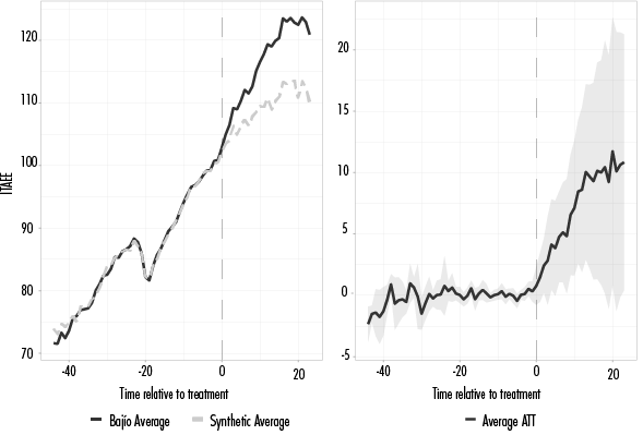
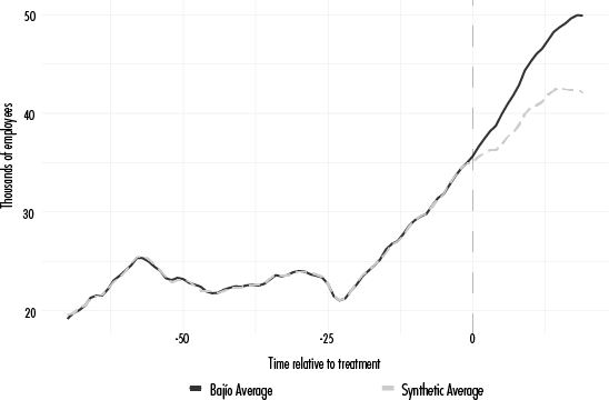
The results are presented according to each assessed dimension of regional development. Although the analysis of the study is conducted on a state level, because of the potential for municipal data in the IMSS information sets, estimates were made on a municipal level for the employment and wage categories. The estimates are presented in two-panel figures. The left panel shows the average observed trends (black series) and synthetic trends (gray series) for the Bajio region for the variable in question. The right panel shows the average treatment effect (ATT) of the variable studied (black series), together with the 90% confidence interval of the estimate (gray shaded area). For the quarterly results, there will be 66 pre-treatment periods, and post-intervention impact is assessed using the ATT for 23 quarters, which is the same post-treatment period as the last treated unit.
The municipal estimates are provided in the annex, which are useful for corroborating the state results and for calculating the potential spillover effects of the automotive industry. Similarly, the annex contains the description of the final models, the matrices of the donor state weights for all synthetic controls and the various robustness tests. Tables A3, A4 and A5 in the annex present balance tables of the pre-treatment averages of the variables of interest and the main covariables for the treated states, the synthetic control group and the donor pool. These allow us to verify the validity of the estimates by finding similar averages between treated states and donors that are part of the positive weighted synthetic controls (synthetic control group).
Total employment
Figure 2 shows the estimate for total employment. We can see that the fit before the intervention is good, and after that slight increases in the ATT trend are noted, which is reflected in the difference of the series in the left panel. During the first quarter, after the establishment of the new automotive companies, an average of at least 4,700 jobs had been created for each state in the Bajío region. After five quarters, average employment increased by 13,000 employees, and by quarter 10, the figure was 36,000. The effect proliferated from quarter 8, with an impact exceeding an average of 122,000 new jobs for the last quarter.

Note: The model presented is the one with the lowest MSE, including the regressions of the dependent variable as explanatory variables.
Source: Compiled by the authors.
Figure 2 Estimated staggered synthetic control for total employment
If we compare the estimates of total employment with respect to new employment originating in the automotive industry, we can conclude that by 2019 an average of more than 122,000 total jobs had been generated in the Bajío region, of which 40,000 corresponded to the total of new direct jobs generated by the assembly plants and indirect jobs in the network of auto part suppliers and other services required by the industry. In other words, there is a differential of at least 82,000 jobs created outside the automotive sector, which indicates the presence of spillover effects of the assemblers on the manufacturing sector or the rest of the economic sectors in the Bajio region.
On aggregate, for 2019, the number of new jobs in all state economies exceeded 638,000. By comparing the two series in the left panel of Figure 2, we can calculate the difference in percentage terms of average employment with respect to its counterfactual. This shows that for 2019 there was an average increase of 15.9% in total employment. The above figure, although informative, hides the heterogeneous effects on a state level. Proportionally, the state of Querétaro registered the most significant impact with an increase of 37.4%, followed by Guanajuato, with a growth of 15.4%.On the other hand, Aguascalientes reported 13.1% new jobs, and finally, the states of Jalisco and San Luis Potosí reported rates of 6.8% and 6.4%, respectively. The results are supported by several empirical studies, which recorded similar results in terms of the effect of industry positioning on aggregate employment growth (Dauth, 2013; Fritsch and Mueller, 2004; Hardjoko et al., 2021).
However, to understand the spillover effects on a territorial level, the methodology was estimated by establishing the specific municipalities that received investment in automotive assembly plants as treated.8The results indicate that by 2019, automotive companies had generated an average of 15,400 new jobs in the municipal economies. This represents an average increase of 20.9% in total employment in the municipalities receiving the investments. Based on the foregoing, 12.6% of the 122,000 jobs generated on a state level originated in the municipalities where the automotive plants were located and, as a result, 87.4% were jobs resulting from territorial spillover effects, which allowed the municipalities of the Bajío region to benefit from the automotive industry.
Manufacturing employment
Considering that most of the new jobs were generated outside the automotive sector, it is important to analyze whether this increase in employment occurred within the manufacturing sector or whether it was displaced to other sectors. The automotive companies' effect on manufacturing sector jobs is presented in Figure 3, which shows that the pre-treatment adjustment is good, with ATT oscillating between zero throughout the period. Once the automotive plants enter the Bajío region, the effect on employment is significant: in the first quarter, an average of 1,344 jobs were generated, which tripled three quarters later, with an increase of 4,820 employees in less than four years. The peak was reached in the last quarter when an estimated 26,500 new jobs were generated.
Pursuant to the foregoing, it is estimated that the balance of new jobs on an industrial level was less than the number of direct and indirect jobs originating from the automotive and auto parts companies.

Note: The model presented is the one with the lowest MSE, including regressions of the dependent variable as explanatory variables.
Source: Compiled by the authors.
Figure 3 Estimated staggered synthetic control for manufacturing employment
In other words, there is a gap which suggests that, during this period, although jobs were generated in manufacturing thanks to automotive production, a significant number of jobs appear to have been lost in other industrial areas. Proportionally, the automotive industry increased manufacturing employment by an average of 14.3% for the states in the Bajío region.9The federal state with the most significant impact was Aguascalientes, with a growth of 20.8%. This was followed by Guanajuato, which received the largest number of assembly plants during this period, with an increase of 16.1%, followed by Querétaro and San Luis Potosí, with increases of 14.2% and 12.4%, respectively. Finally, Jalisco experienced a lower impact, with an increase of only 8.1%.
As far as municipal estimates are concerned (in the annex at the end), it is calculated that, on average for 2019, automotive companies triggered an increase of 7,245 industrial jobs in the municipalities where they were located. This increase in jobs represents an average growth of 30% in manufacturing jobs in the municipalities. Two important points can be deduced from this. First, 46.8% of the total number of jobs created in the municipalities where the automotive companies set up their businesses were in the manufacturing sector, compared with 21.7% on a state level. Second, new regional industrial jobs were concentrated to a greater extent in the municipalities receiving the investments (27.3% of the jobs), compared with new aggregate jobs, of which only 12.6% were created in these municipalities. Therefore, significant spillover effects exist in relation to the municipalities that did not receive the automotive companies.
Quarterly Indicator of State Economic Activity (ITAEE)
Figure 4 shows the estimated impact on economic activity. We can see that, after the intervention, the ATT increased considerably over time: in the first four quarters, the automotive industry managed to increase the ITAEE by an average of 4.14 pp. This impact proliferated, obtaining an increase of 10 pp in quarter 13 and remaining at that level during subsequent periods reaching a peak of 11.74 pp in quarter 20 (2019).
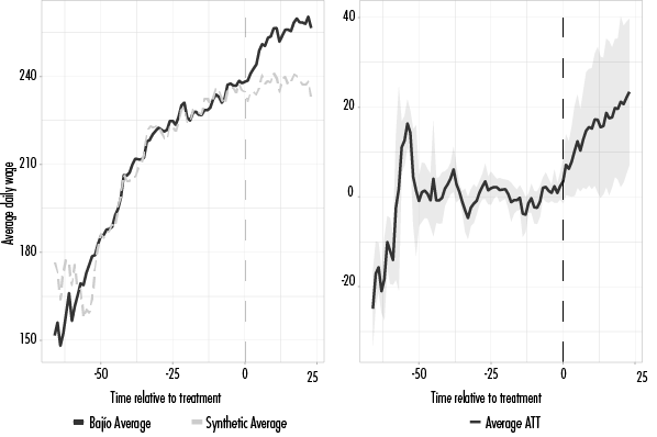
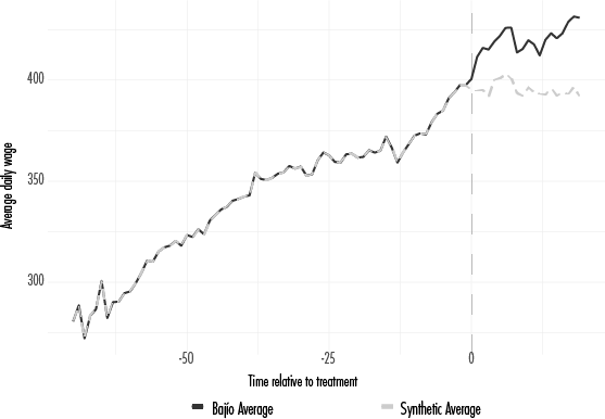
Wages
Taking into account the aforementioned effects on the labor market and on economic activity, it is worth questioning whether this translated into improvements in wages for workers in the region. Therefore, the methodology for the average daily wage was estimated (see Figure 5). We can see that once the automotive companies are established, the ATT trend diverges from zero and grows continuously, reaching an effect greater than MXN$23 for 2019. This indicates that the automotive companies increased the daily wage of Bajío workers by an average of 11.8%. The most significant impact was observed in Queretaro, with an increase of 23.2%, which is consistent with the fact that this territory also registered the most significant expansion in total employment. The results are consistent with the evidence in international literature (Lee and Rodriguez-Pose, 2016).
In-work poverty
We then analyze whether the previous effects were enough to improve social welfare indicators, such as in-work poverty (see figure 6). After the first year of intervention, the assembly companies had managed to reduce in-work poverty by 3.0 pp on average and this effect continued time decreasing by 10.51 pp in 2019. This indicates that had it not been for the establishment of the assembly plants, the Bajío states would have had at least 10 pp more in-work poverty by 2019. This impact is significant in terms of regional development, given that thousands of people were able to escape poverty thanks to the industrial growth of the automotive sector.
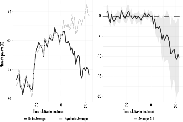
Note: The model presented is the one with the lowest MSE, including employment per capita, average wage, FDI and regressions of the dependent variable as explanatory variables.
Source: Compiled by the authors.
Figure 6 Estimation of the synthetic staggered control for in-work poverty
Had it not been for the investments in the automotive plants, by 2019 all of the Bajío states would have had in-work poverty levels above the national average. Using the counterfactual concept, a static analysis of what would have happened with the in-work poverty ranking is performed (from lowest to highest), if the assembly plants had not been established in the Bajío region (this analysis is summarized in Table 2). The greatest reduction in in-work poverty was recorded in Jalisco, which would have moved from position 6 to 25 in the ranking for lowest in-work poverty if the automotive plants had not been located in its territory. This was followed by San Luis Potosí and Guanajuato, which would have dropped six and five positions, respectively. In the case of San Luis Potosí, this state would have been among the four states with the highest proportion of people subject to in-work poverty. Finally, Aguascalientes and Querétaro would have dropped three positions, surpassing the median of the poorest states.
Figure A6 in the annex shows the behavior of in-work poverty for the five states treated and the average in-work poverty trend for the states that make up the synthetic control. The trend of poverty reduction in the treated states and the marked increase in this indicator for the synthetic control group in the post-treatment period confirms the validity of the estimates and lends veracity to the causal effect described above.
Table 2 Ranking of positions of in work poverty if the automotive companies had not entered the Bajío region
| Satate | ATT | PL 2019 Ranking | Ranking without automobile companies |
| Aguascalientes | -6.90 | 16 | 19 |
| Guanajuato | -7.63 | 13 | 18 |
| Jalisco | -24.93 | 6 | 25 |
| Querétaro | -6.89 | 18 | 21 |
| San Luis Potosí | -8.45 | 23 | 29 |
Source: Compiled by the authors
Enrollment in education
Since industrial plants may increase the demand for workers with a particular level of education, this could be expected to impact the educational enrollment records of the inhabitants of the Bajio region. The annex shows that there is no effect on higher education; however, there is an effect on high school education (see figure 7). In this respect, thanks to the automotive assembly companies, a greater number of young people attended high school, registering an increase in enrollment of 216 new students per ten thousand people in 2018, representing an average increase in enrollment of 3%.

Robustness tests
The results were subjected to various robustness tests, which permitted the assessment of sensitivity to the specification of the synthetic controls, the possible diversity of impacts across federal states, and the potential incidence of the northern and central border states. In the first case, for each dimension of regional development, at least 20 combinations of different models were estimated, including (or excluding) covariables, interactive fixed effects, and fixed effects by treated unit. Second, synthetic controls were again estimated, including three different weights when calculating ATT. Finally, all the estimates were repeated for the automotive states in the northern and central region for the donor set and excluding the states on the territorial borders of the Bajío states. In general, the results obtained are robust, the pre-treatment adjustment and the trends do not experience significant modifications given the different robustness tests, and although some variations occur in the ATT, the direction of the results does not change (results in the annex at the end).
Meanwhile, placebo tests were performed for the final synthetic controls presented in the previous section. The period of the treatment simulating an advance of the impact was changed, and the donor group entered the treated states. In both cases, no impacts are generated by the results, nor do we see trends similar to the true ones.10
5. CONCLUSIONS
This research studied the consequences of the extraordinary growth of the automotive industry in Mexico over the last two decades on regional development. To our knowledge, it is the first causal study to evaluate the impact of the automotive industry on regional development in Mexico, and it contributes to international literature on studies that have analyzed the effects of large industries on development characteristics.
On a state level, the automotive industry increased total employment and manufacturing employment by an average of 15.9% and 14.3%, respectively. The calculations indicate that for every new job created in the automotive sector, an average of 4.97 new jobs were generated in the Bajío state economies. On aggregate, more than 638,000 jobs were created in the territories of the Bajío region, of which 78.3% were created in sectors other than industrial branches. This confirms the extensive spillover effects of the automotive sector, apparently with a much more substantial impact on the service sector.
When assessing impacts within the manufacturing sector, evidence was found of possible job destruction in industrial areas other than the automotive sector, given that the absolute impact on the number of manufacturing jobs was lower than the number of jobs created in automotive and auto parts plants. This is consistent with the concerns of regional development theories in that the arrival of new industries can negatively affect other established industrial branches, generating a displacement effect on economic activity and employment. Despite this, the net employment balance continues to be positive.
The establishment of the automotive industry in the Bajío region promoted local economic development: it increased economic activity, reduced in-work poverty, and increased school enrollment on a high school level. As far as poverty is concerned, according to Fowler and Kleit (2014), its reduction seems to be explained by the fact that the majority of the new jobs are occupied by local workers, who, by obtaining a source of income, can escape the poverty line. The increase in enrollment in education is consistent with the postulates of Porter (1998) and the estimates of Fu and Gabriel (2012), who state that industrial connections continually require increased human capital, so a better supply of education and graduates in the territories would be expected.
Although different variables associated with social development have been analyzed, this paper does not study the responses of state and local governments. These responses could supplement the establishment of automotive plants in the region and explain differences in the results. This paper does not study other specific mechanisms to observe the estimated effects. These questions remain open for future research.
REFERENCES
Abadie, A. (2015). Comparative politics and the synthetic control method. American Journal of Political Science, 59(2). https://doi.org/10.1111/ ajps.12116 [ Links ]
Abadie, A. y Gardeazabal, J. (2003). The economic costs of conflict: A case study of the basque country. The American Economic Review, 93(1). http:// www.jstor.org/stable/3132164 [ Links ]
_________, Diamond, A. y Hainmueller, J. (2007). Synthetic control methods for comparative case studies: Estimating the effect of California’s Tobacco Control Program. Journal of the American Statistical Association, 105(490). https://doi.org/10.1198/jasa.2009.ap08746 [ Links ]
Arrow, K. J. (1962). The economic implications of learning by doing. The Review of Economic Studies, 29(3). https://doi.org/10.2307/2295952 [ Links ]
Asociación Mexicana de la Industria Automotriz (AMIA) (2019). Producción de vehículos ligeros. https://www.amia.com.mx/vehiculosligeros/ [ Links ]
Barnes, T. (2017). Why has the Indian automotive industry reproduced “low road” labour relations? En E. Noronha y P. D’Cruz (eds.), Critical perspectives on work and employment in globalizing India (pp. 37‑56). Springer. https://doi.org/10.1007/978‑981‑10‑3491‑6_3 [ Links ]
Ben‑Michael, E., Feller, A. y Rothstein, J. (2021). Synthetic controls with staggered adoption. Journal of the Royal Statistical Society: Series B (Statistical Methodology), 84(2). https://doi.org/10.1111/rssb.12448 [ Links ]
Carbajal, Y., Almonte, L. de J. y Mejía, P. (2016). La manufactura y la industria automotriz en cuatro regiones de México. Un análisis de su dinámica de crecimiento, 1980‑2014. Economía: Teoría y Práctica, 45. https://doi. org/10.24275/ETYPUAM/NE/452016/Carbajal [ Links ]
Chavarro, A. y Guzmán, L. (2019). Determinantes de la localización de empresas proveedoras automotrices japonesas en la región del Bajío Mexicano. Paradigma Económico, 10(2). https://paradigmaeconomico.uaemex.mx/article/view/11898 [ Links ]
Covarrubias, A. (2017). La geografía del auto en México. ¿Cuál es el rol de las instituciones locales? Estudios Sociales (Hermosillo, Son.), 27(49). http://www.scielo.org.mx/scielo.php?script=sci_abstract&pid=S0188‑45572017000100211&lng=es&nrm=iso&tlng=es [ Links ]
Crossa, M. y Ebner, N. (2020). Automotive global value chains in Mexico: A mirage of development? Third World Quarterly, 41(7). https://doi.org/10. 1080/01436597.2020.1761252 [ Links ]
Dauth, W. (2013). Agglomeration and regional employment dynamics. Papers in Regional Science: The Journal of the Regional Science Association International, 92(2). https://doi.org/10.1111/j.1435‑5957.2012.00447.x [ Links ]
Dube, A. y Zipperer, B. (2015). Pooling multiple case studies using synthetic controls: an application to minimum wage policies (No. 8944). Institute of Labor Economics (IZA). https: //ideas.repec.org/p/iza/izadps/dp8944.html [ Links ]
Fowler, C. S. y Kleit, R. G. (2014). The effects of industrial clusters on the poverty rate: industrial clusters and the poverty rate. Economic Geography, 90(2). https://doi. org/10.1111/ecge.12038 [ Links ]
Fritsch, M. y Mueller, P. (2004). The effects of new business formation on regional development over time. Regional Studies, 38. https://doi. org/10.1080/0034340042000280965 [ Links ]
Fu, Y. y Gabriel, S. A. (2012). Labor migration, human capital agglomeration and regional development in China. Regional Science and Urban Economics, 42(3). https://doi.org/10. 1016/j.regsciurbeco.2011.08.006 [ Links ]
Fujita, M., Krugman, P. R. y Venables, A. (2000). Economía espacial: Las ciudades, las regiones y el comercio internacional. Editorial Ariel. [ Links ]
Haddad, E. A. y Hewings, G. J. (1999). The short‐run regional effects of new investments and technological upgrade in the Brazilian automobile industry: An interregional computable general equilibrium analysis. Oxford Development Studies, 27(3) . https://doi.org/10.1080/13600819908424182 [ Links ]
Hardjoko, A. T., Santoso, D. B., Suman, A. y Sakti, R. K. (2021). The effect of industrial agglomeration on economic growth in East Java, Indonesia. The Journal of Asian Finance, Economics and Business, 8(10). https://doi. org/10.13106/jafeb.2021.vol8.no10.0249 [ Links ]
Instituto Nacional de Estadística y Geografía (INEGI) (2019). Censos Económicos. https://www.inegi.org.mx/programas/ce/2019/ [ Links ]
__________ (2020). Registro administrativo de la industria automotriz de vehículos ligeros y pesados. https://www.inegi.org.mx/datosprimarios/iavl/ [ Links ]
Jacobs, J. (1984). Cities and the wealth of nations: Principles of economic life. Editorial Random House. [ Links ]
Kline, P. y Moretti, E. (2014). Local economic development, agglomeration economies, and the big push: 100 years of evidence from the Tennessee Valley authority. The Quarterly Journal of Economics, 129(1). https://doi.org/10.1093/qje/qjt034 [ Links ]
Krugman, P. (1991). Increasing returns and economic geography. Journal of Political Economy, 99(3). https://doi.org/10.1086/261763 [ Links ]
Larsson, A. (2002). The development and regional significance of the automotive industry: supplier parks in western Europe. International Journal of Urban and Regional Research, 26(4). https://doi.org/10.1111/14682427.00417 [ Links ]
Lee, N. y Rodríguez‑Pose, A. (2016). Is there trickle‑down from tech? Poverty, employment, and the high‑technology multiplier in U.S. cities. Annals of the American Association of Geographers, 106(5). https://doi.org/10.1080/24694452.2016.1184081 [ Links ]
Marshall, A. (1890). Principles of economics. Editorial Macmillan Learning. [ Links ]
Moretti, E. (2010). Local multipliers. American Economic Review, 100(2). https://doi.org/10.1257/aer.100.2.373 [ Links ]
Organización para la Cooperación y el Desarrollo Económico (OECD) (2022). Foreign direct investment statistics: data, analysis and forecasts. https://www.oecd.org/corporate/mne/statistics.htm [ Links ]
Pavlínek, P. (2018). Global production networks, foreign direct investment, and supplier linkages in the integrated peripheries of the automotive industry. Economic Geography , 94(2). https://doi.org/10.1080/00130095.2 017.1393313 [ Links ]
Pavlínek, P., Domański, B. y Guzik, R. (2009). Industrial upgrading through foreign direct investment in Central European automotive manufacturing. European Urban and Regional Studies , 16(1). https://doi. org/10.1177/0969776408098932 [ Links ]
______ y Ženka, J. (2010). Upgrading in the automotive industry: firmlevel evidence from Central Europe. Journal of Economic Geography, 11(3). https://doi.org/10.1093/jeg/lbq023 [ Links ]
______ y Žížalová, P. (2016). Linkages and spillovers in global production networks: Firm‑level analysis of the Czech automotive industry. Journal of Economic Geography, 16(2). https://doi.org/10.1093/jeg/lbu041 [ Links ]
Peyro, M. E., González, M. V. y Hernández, A. (2019). La inversión asiática en el sector automotor de la región del Bajío, México. Expresión Económica, 42. https://doi.org/10.32870/eera.vi42.896 [ Links ]
Porter, M. E. (1998). Clusters and the new economics of competition. Harvard Business Review, 76(6). https://pubmed.ncbi.nlm.nih.gov/10187248/ [ Links ]
Rauch, J. E. (1993). Productivity gains from geographic concentration of human capital: Evidence from the cities. Journal of Urban Economics, 34(3). https://doi.org/10.1006/juec.1993.1042 [ Links ]
Romer, P. M. (1986). Increasing returns and long‑run growth. Journal of Political Economy , 94(5). https://doi.org/10.1086/261420 [ Links ]
Šipikal, M. y Buček, M. (2013). The role of FDIs in regional innovation: Evidence from the automotive industry in Western Slovakia. Regional Science Policy & Practice, 5(4). https://doi.org/10.1111/rsp3.12022 [ Links ]
Turok, I. (1993). Inward investment and local linkages: How deeply embedded is “Silicon Glen?” Regional Studies , 27(5). https://doi.org/10.1080/00 343409312331347655 [ Links ]
1Information obtained from INEGI Economic Censuses between 1999 and 2019, and from the Registro administrativo de la industria automotriz de vehículos ligeros (Administrative Registry for Light Vehicles in the Automotive Industry).
6 It is important to consider that, although the synthetic controls are a weighted average of all the units in the donor pool, the weight of many of them is generally zero, so the group of units that make up a positively weighted synthetic control is generally small.
7 Given that the treatment effects are various, depending on the number of units that receive the treatment, the formula for the average effect on the treated is adjusted for each unit
8 In order to avoid contamination of the synthetic control, all other municipalities in each state were eliminated from the potential donors.
9This result is in line with the estimates of Kline and Moretti (2014) for the case of the United States.
10 These tests are not presented due to their extensive length. However, they are available from the authors upon request.
6. ANNEX
Description of the final models
Tabla A1 Descripción de los modelos finales estimados por dimensión
| Final model | Covariables | Fixed unit effect |
| Total employment | Own regressions | No |
| Manufacturing employment | FDI, own regressions | Yes |
| ITAEE | Unployment rate, FDI, own regressions | Yes |
| Wages | Unployment rate, ITAEE, own regressions | Yes |
| In-work poverty | Employment per capita, average wage, FDI, own regressions | Yes |
| Enrollment in education | GDP public expenditure on education per capita | Yes |
Source: Compiled by the authors
Set of covariables
Table A2 Covariables tested in the estimates, classified by dimensions
| Dimension | Variables |
| Economy | Unemployment rate, employment rate, informality rate, aggregate employment per capita, manufacturing employment per capita, automotive employment per capita, GDP, ITAEE, aggregate FDI, automotive FDI, gross capital formation, rate of change of remittances. |
| Social | Average wage, percentage of employment earning less than minimum wage. |
| Educacation | Education expenditure per capita, secondary school enrollment rate. |
| Health | Health expenditure per capita, social assistance expenditure per capita, public investment in health, crude mortality rate. |
| Security | Homicides and robberies per 100,00 inhabitants. |
| Others | Regressions of the dependent variables in each dimensions evaluated. |
Source: Compiled by the authors
Pre-treatment balance tables
Table A3 Average of the explanatory variables of interest for the pre-treatment period
| State/Variable | Total employment | Manufacturing employment | ITAEE | Wages | In-work poverty | Enrollment in education |
| Aguascalientes | 201 140 | 69 866 | 83.25 | 205.56 | 36.47 | 5 224 |
| Guanajuato | 580 761 | 205 097 | 79.66 | 183.31 | 37.98 | 4 172 |
| Jalisco | 1 126 333 | 307 145 | 83.10 | 158.56 | 29.04 | 4 782 |
| Querétaro | 305 275 | 97 972 | 85.12 | 246.25 | 35.89 | 4 817 |
| San Luis Potosí | 275 793 | 83 428 | 81.54 | 149.29 | 46.97 | 4 633 |
| Average | 497 860 | 152 702 | 82.54 | 188.59 | 37.27 | 4 726 |
| Synthetic control group | 498 372 | 152 676 | 82.20 | 190.26 | 37.91 | 4 731 |
| Donor pool | 459 985 | 118 365 | 87.89 | 193.79 | 37.50 | 5 415 |
Source: Compiled by the authors
Table A4 Average of the main covariables for the pre-treatment period. Section 1
| State/Variable | FDI | Automotive employment per capita | Unemployment rate | Manufacturing employment per capita | Remittances | Total exports |
| Aguascalientes | 63.56 | 1.46% | 5.82% | 6.51% | 2.63 | 1 335 979 |
| Guanajuato | 183.65 | 0.33% | 4.26% | 4.18% | 6.58 | 1 544 099 |
| Jalisco | 316.97 | 0.11% | 3.44% | 4.64% | 10.99 | 3 611 494 |
| Querétaro | 190.09 | 1.16% | 5.19% | 6.63% | 4.50 | 1 447 796 |
| San Luis Potosí | 91.92 | 0.49% | 3.24% | 3.51% | 7.82 | 1 106 370 |
| Average | 169.24 | 0.71% | 4.39% | 5.09% | 6.50 | 1 809 148 |
| Grupo control sintético | 168.62 | 0.63% | 4.66% | 4.07% | 6.52 | 2 092 583 |
| Pool de donantes | 194.15 | 0.38% | 4.12% | 3.36% | 6.89 | 2 063 028 |
Source: Compiled by the authors
Table A5 Average of the mains covariables for the pre-treatment period. Section 2
| State/Variable | Occupation rate | Informality rate | Theft for every 100,000 inhabits | Public expediture on culture and sport (per capita) | Public expediture on education (per capita) | High school enrolment rate |
| Aguascalientes | 55.26% | 24.61% | 124.32 | 343 | 4 024 | 47% |
| Guanajuato | 55.52% | 28.76% | 104.16 | 76 | 973 | 34% |
| Jalisco | 60.94% | 27.40% | 122.64 | 33 | 830 | 40% |
| Querétaro | 54.60% | 22.33% | 136.13 | 61 | 3 823 | 45% |
| San Luis Potosí | 56.85% | 24.91% | 99.52 | 92 | 2 940 | 41% |
| Average | 56.64% | 25.60% | 117.35 | 121 | 2 518 | 42% |
| Grupo control sintético | 56.99% | 25.63% | 114.97 | 60 | 2 503 | 47% |
| Pool de donantes | 57.94% | 26.83% | 138.97 | 105 | 2 828 | 49% |
Source: Compiled by authors
Estimated enrolment in undergraduate education
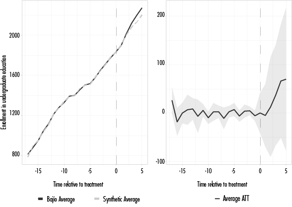
Source: Compiled by the authors
Figure A1 Staggered synthetic control estimate for enrolment in undergraduate education per ten thousand people aged 18 to 24

Source: Compiled by the authors
Figure A2 Staggered synthetic control for total municipal employment
Source: Compiled by the authors
Figure A3 Staggered synthetic control for municipal manufacturing employment
Source: Compiled by the authors
Figure A4 Synthetic staggered control for the average municipal wage
Table A6 Matrix of donor state weights in the staggered synthetic control for total employment
| Donor state | Treated state | ||||
| Aguascalientes | Guanajuato | Jalisco | Querétaro | San Luis Potosí | |
| Aguascalientes | 0.00 | 0.00 | 0.00 | 0.00 | 0.00 |
| Baja California Sur | 0.55 | 0.00 | 0.00 | 0.00 | 0.33 |
| Campeche | 0.00 | 0.00 | 0.00 | 0.00 | 0.00 |
| Chiapas | 0.00 | 0.03 | 0.00 | 0.02 | 0.00 |
| Ciudad de México | 0.00 | 0.05 | 0.10 | 0.05 | 0.01 |
| Colima | 0.27 | 0.00 | 0.00 | 0.00 | 0.00 |
| Durango | 0.16 | 0.00 | 0.00 | 0.00 | 0.00 |
| Guanajuato | 0.00 | 0.00 | 0.00 | 0.00 | 0.00 |
| Guerrero | 0.00 | 0.00 | 0.00 | 0.00 | 0.00 |
| Hidalgo | 0.00 | 0.00 | 0.00 | 0.03 | 0.00 |
| Jalisco | 0.00 | 0.00 | 0.00 | 0.00 | 0.00 |
| Michoacán | 0.00 | 0.00 | 0.00 | 0.00 | 0.16 |
| Nayarit | 0.00 | 0.00 | 0.00 | 0.00 | 0.00 |
| Oaxaca | 0.00 | 0.00 | 0.00 | 0.00 | 0.01 |
| Querétaro | 0.00 | 0.00 | 0.03 | 0.00 | 0.00 |
| Quintana Roo | 0.00 | 0.49 | 0.15 | 0.36 | 0.00 |
| San Luis Potosí | 0.00 | 0.00 | 0.00 | 0.00 | 0.00 |
| Sinaloa | 0.00 | 0.00 | 0.00 | 0.00 | 0.00 |
| Tabasco | 0.00 | 0.15 | 0.00 | 0.52 | 0.22 |
| Tamaulipas | 0.02 | 0.23 | 0.32 | 0.02 | 0.01 |
| Tlaxcala | 0.00 | 0.00 | 0.00 | 0.00 | 0.00 |
| Veracruz | 0.00 | 0.00 | 0.39 | 0.00 | 0.00 |
| Yucatán | 0.00 | 0.00 | 0.00 | 0.00 | 0.20 |
| Zacatecas | 0.00 | 0.04 | 0.00 | 0.00 | 0.05 |
Source: Compiled by the authors
Table A7 Matrix of weights of donor states for manufacturing employment
| Donor state | Treated state | ||||
| Aguascalientes | Guanajuato | Jalisco | Querétaro | San Luis Potosí | |
| Aguascalientes | 0.00 | 0.00 | 0.22 | 0.00 | 0.00 |
| Baja California Sur | 0.16 | 0.00 | 0.00 | 0.00 | 0.37 |
| Campeche | 0.00 | 0.00 | 0.00 | 0.23 | 0.00 |
| Chiapas | 0.00 | 0.00 | 0.00 | 0.00 | 0.00 |
| Ciudad de México | 0.00 | 0.00 | 0.00 | 0.00 | 0.00 |
| Colima | 0.00 | 0.00 | 0.00 | 0.10 | 0.03 |
| Durango | 0.00 | 0.00 | 0.00 | 0.00 | 0.28 |
| Guanajuato | 0.00 | 0.00 | 0.00 | 0.00 | 0.00 |
| Guerrero | 0.00 | 0.00 | 0.00 | 0.00 | 0.00 |
| Hidalgo | 0.21 | 0.00 | 0.00 | 0.07 | 0.00 |
| Jalisco | 0.00 | 0.00 | 0.00 | 0.00 | 0.00 |
| Michoacán | 0.62 | 0.00 | 0.14 | 0.00 | 0.00 |
| Nayarit | 0.00 | 0.00 | 0.00 | 0.00 | 0.00 |
| Oaxaca | 0.00 | 0.00 | 0.00 | 0.00 | 0.00 |
| Querétaro | 0.00 | 0.00 | 0.00 | 0.00 | 0.00 |
| Quintana Roo | 0.00 | 0.00 | 0.00 | 0.00 | 0.00 |
| San Luis Potosí | 0.00 | 0.00 | 0.00 | 0.00 | 0.00 |
| Sinaloa | 0.00 | 0.42 | 0.00 | 0.00 | 0.19 |
| Tabasco | 0.00 | 0.00 | 0.00 | 0.00 | 0.12 |
| Tamaulipas | 0.00 | 0.00 | 0.00 | 0.00 | 0.00 |
| Tlaxcala | 0.00 | 0.28 | 0.00 | 0.00 | 0.00 |
| Veracruz | 0.00 | 0.29 | 0.00 | 0.00 | 0.00 |
| Yucatán | 0.00 | 0.00 | 0.64 | 0.00 | 0.00 |
| Zacatecas | 0.00 | 0.00 | 0.00 | 0.60 | 0.00 |
Source: Compiled by the authors
Table A8 Matrix of weights of donor states in the staggered synthetic control for the ITAEE
| Donor state | Treated state | ||||
| Aguascalientes | Guanajuato | Jalisco | Querétaro | San Luis Potosí | |
| Aguascalientes | 0.00 | 0.00 | 0.14 | 0.00 | 0.00 |
| Baja California Sur | 0.00 | 0.00 | 0.00 | 0.00 | 0.14 |
| Campeche | 0.00 | 0.00 | 0.00 | 0.00 | 0.02 |
| Chiapas | 0.00 | 0.08 | 0.00 | 0.00 | 0.00 |
| Ciudad de México | 0.04 | 0.01 | 0.13 | 0.08 | 0.00 |
| Colima | 0.24 | 0.00 | 0.05 | 0.05 | 0.00 |
| Durango | 0.00 | 0.34 | 0.20 | 0.00 | 0.24 |
| Guanajuato | 0.00 | 0.00 | 0.00 | 0.00 | 0.00 |
| Guerrero | 0.00 | 0.00 | 0.00 | 0.00 | 0.00 |
| Hidalgo | 0.00 | 0.00 | 0.00 | 0.00 | 0.08 |
| Jalisco | 0.00 | 0.00 | 0.00 | 0.00 | 0.00 |
| Michoacán | 0.00 | 0.00 | 0.00 | 0.00 | 0.00 |
| Nayarit | 0.00 | 0.00 | 0.00 | 0.00 | 0.13 |
| Oaxaca | 0.00 | 0.00 | 0.00 | 0.00 | 0.00 |
| Querétaro | 0.00 | 0.00 | 0.23 | 0.00 | 0.00 |
| Quintana Roo | 0.00 | 0.00 | 0.00 | 0.24 | 0.01 |
| San Luis Potosí | 0.00 | 0.00 | 0.00 | 0.00 | 0.00 |
| Sinaloa | 0.00 | 0.00 | 0.00 | 0.00 | 0.00 |
| Tabasco | 0.16 | 0.00 | 0.22 | 0.55 | 0.00 |
| Tamaulipas | 0.40 | 0.52 | 0.00 | 0.09 | 0.12 |
| Tlaxcala | 0.01 | 0.05 | 0.00 | 0.00 | 0.05 |
| Veracruz | 0.00 | 0.00 | 0.02 | 0.00 | 0.00 |
| Yucatán | 0.00 | 0.00 | 0.00 | 0.00 | 0.21 |
| Zacatecas | 0.15 | 0.00 | 0.00 | 0.00 | 0.00 |
Source: Compiled by the authors
Table A9 Matrix of weights of donor states in the staggered synthetic control salary
| Donor state | Treated state | ||||
| Aguascalientes | Guanajuato | Jalisco | Querétaro | San Luis Potosí | |
| Aguascalientes | 0.00 | 0.00 | 0.00 | 0.00 | 0.00 |
| Baja California Sur | 0.02 | 0.00 | 0.23 | 0.00 | 0.00 |
| Campeche | 0.00 | 0.00 | 0.00 | 0.00 | 0.00 |
| Chiapas | 0.00 | 0.00 | 0.00 | 0.00 | 0.00 |
| Ciudad de México | 0.00 | 0.08 | 0.00 | 0.00 | 0.00 |
| Colima | 0.00 | 0.11 | 0.00 | 0.42 | 0.00 |
| Durango | 0.00 | 0.00 | 0.00 | 0.00 | 0.03 |
| Guanajuato | 0.00 | 0.00 | 0.00 | 0.00 | 0.00 |
| Guerrero | 0.00 | 0.00 | 0.00 | 0.00 | 0.00 |
| Hidalgo | 0.00 | 0.15 | 0.00 | 0.00 | 0.00 |
| Jalisco | 0.00 | 0.00 | 0.00 | 0.00 | 0.00 |
| Michoacán | 0.00 | 0.00 | 0.00 | 0.00 | 0.00 |
| Nayarit | 0.00 | 0.00 | 0.00 | 0.00 | 0.00 |
| Oaxaca | 0.00 | 0.00 | 0.13 | 0.00 | 0.00 |
| Querétaro | 0.00 | 0.00 | 0.08 | 0.00 | 0.00 |
| Quintana Roo | 0.29 | 0.00 | 0.09 | 0.00 | 0.05 |
| San Luis Potosí | 0.00 | 0.00 | 0.00 | 0.00 | 0.00 |
| Sinaloa | 0.00 | 0.00 | 0.00 | 0.00 | 0.00 |
| Tabasco | 0.00 | 0.13 | 0.00 | 0.00 | 0.24 |
| Tamaulipas | 0.68 | 0.17 | 0.00 | 0.57 | 0.20 |
| Tlaxcala | 0.00 | 0.00 | 0.00 | 0.01 | 0.00 |
| Veracruz | 0.00 | 0.00 | 0.00 | 0.00 | 0.00 |
| Yucatán | 0.00 | 0.00 | 0.00 | 0.00 | 0.00 |
| Zacatecas | 0.00 | 0.36 | 0.46 | 0.00 | 0.48 |
Source: Compiled by the authors
Table A10 Matrix of weights of donor states in the staggered synthetic control for in-work poverty
| Donor state | Treated entity | ||||
| Aguascalientes | Guanajuato | Jalisco | Querétaro | San Luis Potosí | |
| Aguascalientes | 0.00 | 0.00 | 0.00 | 0.00 | 0.00 |
| Baja California Sur | 0.00 | 0.00 | 0.00 | 0.11 | 0.00 |
| Campeche | 0.00 | 0.00 | 0.00 | 0.17 | 0.00 |
| Chiapas | 0.00 | 0.00 | 0.08 | 0.00 | 0.00 |
| Ciudad de México | 0.11 | 0.03 | 0.05 | 0.14 | 0.00 |
| Colima | 0.33 | 0.45 | 0.21 | 0.00 | 0.00 |
| Durango | 0.00 | 0.01 | 0.04 | 0.00 | 0.00 |
| Guanajuato | 0.00 | 0.00 | 0.00 | 0.00 | 0.00 |
| Guerrero | 0.00 | 0.11 | 0.00 | 0.00 | 0.07 |
| Hidalgo | 0.10 | 0.06 | 0.00 | 0.00 | 0.00 |
| Jalisco | 0.00 | 0.00 | 0.00 | 0.00 | 0.00 |
| Michoacán | 0.00 | 0.16 | 0.00 | 0.14 | 0.00 |
| Nayarit | 0.00 | 0.00 | 0.00 | 0.00 | 0.00 |
| Oaxaca | 0.00 | 0.04 | 0.00 | 0.00 | 0.01 |
| Querétaro | 0.00 | 0.00 | 0.00 | 0.00 | 0.00 |
| Quintana Roo | 0.00 | 0.00 | 0.00 | 0.19 | 0.00 |
| San Luis Potosí | 0.00 | 0.00 | 0.00 | 0.00 | 0.00 |
| Sinaloa | 0.14 | 0.00 | 0.61 | 0.00 | 0.00 |
| Tabasco | 0.00 | 0.00 | 0.00 | 0.19 | 0.00 |
| Tamaulipas | 0.05 | 0.00 | 0.00 | 0.00 | 0.08 |
| Tlaxcala | 0.00 | 0.15 | 0.00 | 0.06 | 0.28 |
| Veracruz | 0.00 | 0.00 | 0.00 | 0.00 | 0.15 |
| Yucatán | 0.00 | 0.00 | 0.01 | 0.00 | 0.40 |
| Zacatecas | 0.27 | 0.00 | 0.00 | 0.00 | 0.00 |
Source: Compiled by the authors
Table A11 Matrix of weights of donor states for high school enrollment
| Donor state | Treated entity | ||||
| Aguascalientes | Guanajuato | Jalisco | Querétaro | San Luis Potosí | |
| Aguascalientes | 0.00 | 0.00 | 0.00 | 0.00 | 0.00 |
| Baja California Sur | 0.00 | 0.00 | 0.00 | 0.00 | 0.00 |
| Campeche | 0.00 | 0.00 | 0.00 | 0.00 | 0.00 |
| Chiapas | 0.00 | 0.00 | 0.00 | 0.00 | 0.00 |
| Ciudad de México | 0.03 | 0.00 | 0.09 | 0.00 | 0.00 |
| Colima | 0.00 | 0.00 | 0.00 | 0.00 | 0.00 |
| Durango | 0.00 | 0.00 | 0.00 | 0.00 | 0.12 |
| Guanajuato | 0.00 | 0.00 | 0.00 | 0.00 | 0.00 |
| Guerrero | 0.13 | 0.00 | 0.13 | 0.00 | 0.00 |
| Hidalgo | 0.00 | 0.00 | 0.00 | 0.00 | 0.39 |
| Jalisco | 0.00 | 0.00 | 0.00 | 0.00 | 0.00 |
| Michoacán | 0.00 | 0.00 | 0.00 | 0.00 | 0.39 |
| Nayarit | 0.00 | 0.00 | 0.00 | 0.16 | 0.00 |
| Oaxaca | 0.00 | 0.15 | 0.00 | 0.16 | 0.10 |
| Querétaro | 0.00 | 0.00 | 0.00 | 0.00 | 0.00 |
| Quintana Roo | 0.44 | 0.00 | 0.00 | 0.04 | 0.00 |
| San Luis Potosí | 0.00 | 0.00 | 0.00 | 0.00 | 0.00 |
| Sinaloa | 0.00 | 0.00 | 0.04 | 0.00 | 0.00 |
| Tabasco | 0.00 | 0.00 | 0.00 | 0.00 | 0.00 |
| Tamaulipas | 0.00 | 0.00 | 0.00 | 0.31 | 0.00 |
| Tlaxcala | 0.38 | 0.00 | 0.00 | 0.00 | 0.00 |
| Veracruz | 0.00 | 0.00 | 0.15 | 0.15 | 0.00 |
| Yucatán | 0.00 | 0.85 | 0.58 | 0.00 | 0.00 |
| Zacatecas | 0.00 | 0.00 | 0.00 | 0.17 | 0.00 |
Source: Compiled by the authors
Robustness tests
Sensitivity to the specification
Table A12 Results of the average ATT for the robustness test using sensitivity to model specifications
| Dimension | ATT M.F. | ATT M.2 | ATT M.3 | ATT M.4 | ATT M.5 |
| Total employment | 57.27 | 46.56 | 46.78 | 51.44 | 49.64 |
| Manufacturing employment | 13.91 | 19.47 | 19.98 | 18.74 | 18.39 |
| ITAEE | 7.09 | 5.63 | 5.48 | 5.34 | 5.83 |
| Wages | 13.39 | 13.96 | 13.85 | 14.15 | 14.47 |
| In-work poverty | -5.33 | -5.24 | -5.36 | -5.27 | -5.28 |
| Enrollment in high school | 167.23 | 159.43 | 158.53 | 155.17 | 149.28 |
Note: The second column corresponds to the estimates of the final model presented in the results section, while the remaining four columns are, in respective order, the following four models with lower MSE.
Source: Compiled by authors
Differences in impacts
Table A13 ATT results for robustness tests, including weights to capture different effects across states
| Dimensión | ATT M.F. | ATT pesos PIB | ATT pesos UE | ATT pesos empleo |
| Total employment | 57.27 | 80.37 | 65.38 | 64.29 |
| Manufacturing employment | 13.91 | 15.87 | 14.69 | 14.94 |
| ITAEE | 7.09 | 6.34 | 6.48 | 6.67 |
| Wages | 13.39 | 9.89 | 13.72 | 11.46 |
| In-work poverty | -5.33 | -4.19 | -5.52 | -4.17 |
| Enrollment in high school | 167.23 | 127.49 | 175.31 | 158.34 |
Note: the second column shows the ATT of the final model and the remaining columns are the ATT with weights of GDP, economic units and employed personnel in the respective order.
Source: Compiled by the authors.
Robustness test with state units similar to those treated
Table A14 ATT results for robustness test including as donors exclusively the state units similar to the treated ones
| Dimensión | ATT M.1 | ATT M.2 | ATT M.3 |
| Total employment | 56.81 | 57.50 | 52.28 |
| Manufacturing employment | 13.38 | 16.87 | 14.54 |
| ITAEE | 7.21 | 6.65 | 6.93 |
| Wages | 14.74 | 16.12 | 15.84 |
| In-work poverty | -5.46 | -4.91 | -4.97 |
| Enrollment in high school | 155.59 | 148.24 | 159.50 |
Note: The second column shows the ATT of the initial model without eliminating possible donors. The third column estimates the ATT by eliminating the 12 states least similar to those treated (in terms of GDP per capita), while the fourth column presents the ATT of each model, eliminating the 16 states least similar to those treated (in terms of GDP per capita).
Source: Compiled by the authors.
Robustness test excluding possibly affected states from the donor group
Table A15 ATT results for robustness test excluding from the donor group the federal states of the country possibly affected by the treatment
| Dimension | ATT M.1 | ATT M.2 | ATT M.3 | ATT M.4 |
| Total employment | 56.81 | 59.43 | 57.27 | 58.89 |
| Manufacturing employment | 13.38 | 15.64 | 13.91 | 12.81 |
| ITAEE | 7.21 | 6.93 | 7.09 | 7.16 |
| Wages | 14.74 | 15.85 | 13.39 | 13.75 |
| In-work poverty | -5.46 | -4.98 | -5.33 | -4.95 |
| Enrollment in high school | 155.59 | 143.94 | 167.23 | 187.87 |
Note: The second column shows the ATT of the initial model without eliminating possible donors. The third column estimates the ATT by eliminating the northern automotive state from the group of donors, while the fourth column presents the ATT of each model, eliminating both the northern and central automotive states (final model shown in the results). The fifth column excludes the states territorially bordering the treated states of the Bajío region.
Source: Compiled by the authors.
Non-automotive manufacturing employment

Source: Compiled by the authors
Figure A5 Synthetic control for non-automotive manufacturing employment

Received: July 22, 2022; Accepted: January 30, 2023
 Este es un artículo publicado en acceso abierto bajo una licencia Creative Commons
