


Services on Demand
Journal
Article
 text in
  English (pdf)
 Article in xml format
 Article references
 Send this article by e-mail
Indicators
-
 Cited by SciELO
 -
 Access statistics
Related links
-
 Similars in
SciELO
Similars in
SciELO
Share

 Permalink
Problemas del desarrollo
Print version ISSN 0301-7036
Prob. Des vol.54 n.212 Ciudad de México Jan./Mar. 2023 Epub Aug 14, 2023
https://doi.org/10.22201/iiec.20078951e.2023.212.69916
Articles
Potential economic impacts of climate change on livestock: the case of Mexico
a Universidad Nacional Autónoma de México (UNAM) - Faculty of Economics, México. Email addresses: sbasurto@economia. unam.mx y gapaliza@unam.mx, respectivamente.
b UNAM Faculty of Medicine, Veterinary and Zootechnics, Mexico. Email address: juliariosmohar@gmail.com.
This article identifies the impacts of climate change on livestock production in Mexico. Data from 28,337 livestock production units is used to estimate a Ricardian model and simulate the effects of climate change on net income per head. The main results suggest that climate change could reduce net income between -13.42 and -16.87% in 2041-2060 and between -14.42 and -33.83% in 2081-2100. Furthermore, small, less diversified producers appear to be the most vulnerable to climate change.
Keywords: change; livestock; Ricardian model
El objetivo del presente artículo es identificar los impactos del cambio climático en la ganadería en México. Se utiliza información correspondiente a 28 337 unidades de producción ganadera para estimar un modelo Ricardiano y simular los impactos del cambio climático en los ingresos netos por cabeza. Los principales resultados sugieren que el cambio climático podría reducir los ingresos netos entre -13.42 y -16.87% en 2041-2060 y entre -14.42 y -33.83% en 2081-2100. Además, los productores pequeños y con menor diversificación parecen ser los más vulnerables al cambio climático.
Palabras clave: cambio climático; ganadería; modelo Ricardiano
Clasificación JEL: Q12; Q15; Q54
1. INTRODUCTION
In 2020, the Food and Agriculture Organization of the United Nations (FAO) reported stocks of 1,526 and 953 million heads of cattle and pigs in the world, respectively and annual production of 68, 110 and 718 million tons of beef, pork and milk, respectively (FAO, 2022). Although the average yearly growth rates of cattle, swine, beef, pork and milk production stocks have been 0.82, 1.46, 1.53, 2.56 and 1.41% during the period 1961-2020, the expected growth in demand for animal food for the following years may not be in line with supply.
According to estimates by the United Nations (UN) Department of Economic and Social Affairs, the global population is expected to reach 9.74 billion people by 2050, and the number of people living in the world by 2050 is expected to rise to 9.74 billion and 10.88 billion people in 21001(UN, 2019). The Organization for Economic Co-operation and Development (OECD) reports that per capita consumption of beef,2pork3and milk was 6.63 kg, 11.48 kg and 9 kg4from 1990-2020 (OECD, 2021). If this per capita consumption is maintained and the world population increases by 3.08 billion people by 21005, annual beef, pork and milk production would have to increase by 39.52% at current levels. In Mexico, the Sistema de Información Agroalimentaria de Consulta (SIACON) indicates that in 2020 cattle and swine stocks were 8.41 and 20.29 million heads respectively. Likewise, the annual production of beef, pork and milk amounts to 2.08, 1.65 million tons and 12.56 billion liters (SADER, 2021). Similar to global trends, the average annual growth rates of beef, pork and milk production were 1.69, 0.70 and 1.57% during the period 1980-2020 and by 2050 and 2100, the population in Mexico is expected to be 151.15 and 141.51 million people (UN, 2019). Therefore, if per capita consumption levels were to remain fixed, the supply of beef, pork and milk, either by means of domestic production or imports, would have to increase by 20.33 and 9.75% in 2050 and 2100 in relation to 2020 levels.6
To close the gap between supply and demand for livestock products in the coming years, more natural resources or technological changes will need to be incorporated into the production process, making it possible to increase production using fewer inputs. Furthermore, climate change will impose an additional challenge on the sector to close the gap between supply and demand. On a global level, the Intergovernmental Panel for Climate Change (IPCC) estimates that global surface temperatures will increase by between 1.2 °C and 3.0 °C in 2041-2060 and between 1.0 °C and 5.7 °C in 2081-2100 compared with the period 1850-1900, depending on the Greenhouse Gas (GHG) emissions scenario used, or Shared Socioeconomic Pathway (SSP) (IPCC, 2021). In Mexico, the Global Climate Model (GCM) ACCESS-ESM1-5 estimates that the change in average temperature will be between 1.79 °C and 3.72 °C in 2041-2060, between 1.79 °C and 3.72 °C in 2041-2060 and between 1.86 °C and 7.05 °C in 2081-2100 (Fick and Hijmans, 2017)7. The increase in global surface temperature may affect production conditions in the livestock sector due to increased proliferation of pests and disease, alteration of the hydrological cycle and water availability, the availability of feed and increased costs resulting from strategies to adapt to the new climate conditions.
According to the GCM ACCESS-ESM1-5, in municipalities where some livestock activity was reported in the 2014 National Agricultural Survey (ENA 2014) (INEGI, 2014a) from the National Institute of Statistics and Geography (INEGI), the temperature is expected to increase between 2.10 °C and 2.84 °C in 2041-2060 and between 2.18 °C and 5.25 °C in 2081-2100 and rainfall could decrease between -0.99 mm/month (1.32%) and -6.52 mm/month (8.71%) between 2041 and 2060 and between -1.26 mm/month (1.68%) and -17.02 mm/month (22.74%) for the period 2081-2100, depending on the history of GHG accumulation in the atmosphere (Fick and Hijmans, 2017).
Based on the foregoing, this research identifies the impacts of these changes on livestock production in Mexico and, in doing so, it contributes to existing literature: i) with the first study in Mexico using the Ricardian model proposed by Mendelsohn et al. (1994), to estimate the impacts of climate change on the livestock sector; ii) by presenting the heterogeneity of impacts among different types of livestock producers; and, iii) by using a larger sample of Production Units (PU), in terms of observations, than those found in international literature.
The Ricardian model, with which the association between climate and net income is identified, uses information from 28,337 livestock PUs, reporting their location in the 2014 ENA. The location of the PU permits the linking of Geographical Information Systems (GIS) for climate and other variables with the information from the ENA 2014. Thus, it was possible to construct a database containing net income per head of cattle, temperature, rainfall, temperature variation, rainfall variation and socio-demographic characteristics of the producers.
The results indicate that, on average, an additional 1°C (1mm/month) of temperature (rainfall) is associated with an MXN$118.5 (MXN$21.1) decrease in net income per head of cattle. Using the expected values for temperature and rainfall levels in the period 2081-2100, it is estimated that climate change may decrease net income by between MXN$289 and MXN$678 per head, or between 14.42 and 33.83% of the current level.
For a better understanding of the research, the article is structured as follows: after the introduction, section 2 presents a synthesis of the literature review on studies that take into consideration a Ricardian model to identify the impacts of climate change on livestock on an international level. Section 3 describes the theory, methodology and statistical information used to determine the effects of climate change on livestock production in Mexico. Section 4 presents estimates of the Ricardian model for different samples, estimates of changes in livestock income according to different climate change scenarios and a discussion of the implications of the results. Section 5 provides the conclusions.
2. REVIEW OF THE LITERATURE PREVIOUS STUDIES
In recent years, the Ricardian model has become popular because it takes into consideration the adaptation processes of producers in relation to different climate conditions and their capacity to incorporate the diversity that exists between PUs. This represents an advantage over agronomic models because the latter do not consider adaptation and, consequently, overestimate the impacts of climate change on the agricultural sector. Likewise, computable general equilibrium models typically use aggregated information, thus failing to include diversity among producers (Mendelsohn and Dinar, 2009).
The Ricardian model is used to quantify the impacts of climate change on agriculture and livestock. In the livestock sector, there are studies for Africa (Seo and Mendelsohn, 2007a, 2007b; Seo and Mendelsohn, 2008a, 2008b, 2008d); South America (Mendelsohn and Seo, 2007; Seo and Mendelsohn, 2008c; Seo, 2016); Kenya (Kabubo-Mariara, 2009); Mongolia (Batsuuri and Wang, 2017); Ethiopia (Gebreegziabher et al., 2013) and South Africa (Tibesigwa et al., 2017), which consider beef cattle, dairy cattle, sheep, poultry and goats.
Previous studies have used different indicators to quantify Ricardian or dependent variable income. Within the set of estimates for livestock, it is found that livestock income can be estimated by calculating net income per PU, net income per head, land value per hectare, land value per PU and the value of livestock per PU. In extensive livestock farming or free grazing, it is difficult to determine the area used to feed livestock, especially in regions with ejido or communal lands, so the net income or value of the land per unit area is often not used. Therefore, a significant proportion of articles use the value of the dependent variable per animal or PU. The need for more information regarding land tenure and property rights encourages the use of the net income variable instead of land value, especially in countries or regions with weak land markets (Mendelsohn and Dinar, 2009).
The Ricardian model for livestock includes a broad set of control variables. Most studies use the altitude at which the PU is located, whether it has electricity, the type of livestock, product sales prices, size of the producer's household, percentage of grassland in the region, years of education of the producer, population density and access to credit. Less frequently, variables such as distance to input and output markets, distance to the nearest port, training programs and producer experience are observed. Regarding the level of aggregation, in 94.73% of the studies, the unit of analysis is the PU or farm, and the range of observations in the Ricardian models using this level of aggregation goes from 214 to 15,002 farms. Due to the vast diversity between livestock producers, it is observed that the R-squared of the Ricardian models ranges between 0.08 and 0.75, with an average value of 0.2.
When considering those estimates in which sufficient information is available to obtain the proportion of the marginal effects on the value of the dependent variable, it is found that the range of these proportions is extensive. In the case of temperature, an additional degree Celsius would generate a change of between -113 and 112% of the dependent variable8with a mean value of 13.84% and a median of 0.68%9. For rainfall, an additional mm/month could cause a change of between -28 and 5% of the dependent variable and a mean value of -3.63% and median of -0.8% (Seo and Mendelsohn, 2008a; Gebreegziabher et al., 2013; Van Passel et al., 2017; Tibesigwa et al., 2017; Bozzola et al., 2018). According to previous research, the marginal effects of temperature and rainfall on livestock income are diverse, and both the sign and magnitude depend on factors such as the location of the PU, the value of the current climate and the species considered in the estimation of the Ricardian model.
According to different climate change scenarios for Africa, Seo and Mendelsohn (2008b) estimate changes between -35.22 and 153.6%, Seo and Mendelsohn (2008a) between -26.4 and 322.9%, Seo and Mendelsohn (2008d) between -8.08 and 168%, and Seo and Mendelsohn (2007b) between -72.8 and -41.7% of net livestock income by the end of the century compared with current levels. For Latin America, Seo and Mendelsohn (2008c) estimate changes of between -187 and 38% in the value of PU livestock land by 2100. In South America, Seo (2016) estimates a gain of 59.45% and Mendelsohn and Seo (2007) estimate changes between -19.48 and 54.81% in land value in 2100 as a consequence of climate change. Country-level studies indicate that net livestock incomes in Kenya could decline between -169 and 38% (Kabubo-Mariara, 2009); in Mongolia, such changes would range between -80.7 and 42.4% (Batsuuri and Wang, 2017); in Ethiopia between -112 and 188% (Gebreegziabher et al., 2013); and in South Africa between -133.3 and 6.1% (Tibesigwa et al., 2017) by 2100, compared with current levels. Based on estimates from previous studies, climate change will have heterogeneous effects on the net income or value of PU livestock land.
For agriculture in Mexico, three studies use the Ricardian model to estimate the impacts of climate change. Mendelsohn et al. (2010) use information from 621 rural households where the main activity is agriculture to evaluate these impacts and livestock activities are not the central part of the analysis. Galindo et al. (2015) use a panel of data on a municipal level to estimate the impacts of climate change on the agricultural sector without considering livestock activities. Basurto-Hernandez (2019) estimates a Ricardian model for the entire livestock sector but does not break down the heterogeneous effects by producer type or present estimates of the potential impacts of climate change on livestock production. Based on the foregoing, the literature review indicates no similar study in Mexico for livestock.
3. RICARDIAN MODELING AND STATISTICAL INFORMATION
The Ricardian model assumes that producerimaximizes their net income in periodt,taking into consideration the product and input prices prevailing in the market during the corresponding period. Based on this information and the long-term climate, or climate expectation, the producer chooses the livestock species that generates the highest net income. The foregoing can be expressed as follows:
where
is the production of species
Thus, the Ricardian function originates from the optimization process described in expression (1) and captures the association between the variation of net income and the variation of the exogenous variables that influence the optimization process, i.e., the Ricardian model is the reduced form11of the net income function. The impact of climate change can be obtained using the Ricardian model defined in expression (2) as follows:
where
where
Furthermore, the effect of climate change on net income for each PU can be obtained using the following formula:
where subscript 1 indicates the value of the variable pursuant to different climate change scenarios and subscript 0 is the current value of the corresponding variable.
To estimate the different specifications of the Ricardian model defined in equation (4), we use economic and geographic location information from 28,337 PU reported in the ENA 2014 (INEGI, 2014a).15The dependent variable is net income per head of cattle and results from calculating the quotient of the difference of income16and expenses17over the number of head of cattle and pigs18in the PU.19
Figure 1 shows the mean net income and standard deviation per PU and head of cattle for each sample percentile. 39.37% of the producers in the sample have negative net income. In general, the PUs with negative values have the same climate, the household size is the same and the age and education of the producer are similar to the rest of the producers. However, a higher proportion of indigenous, female and small producers in PUs leads to negative net income. Likewise, there is also a lower percentage of beneficiaries from the Livestock Development Program (PROGAN)20in the group of producers, with negative net income (8.22% of everyone in this group) compared to those with positive net income (26.47% of everyone in this group).
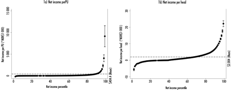
Note: the dots represent the mean net income of the corresponding percentile, while the line above and below each dot represents the standard deviation. Source: Prepared by the authors with data from the National Agricultural Survey (INEGI, 2014a).
Figure 1 Mean net income and standard deviation by percentile
According to the literature review described above, the Ricardian model's control variables comprise temperature and rainfall averages, climate variation, socio-demographic characteristics of producers and other exogenous variables that determine net income in the livestock sector.
To obtain the temperature and rainfall averages, the standard deviation of temperature, the variation coefficient in rainfall and daytime temperature, we used the raster databases (matrix of cells or pixels) published by Fick and Hijmans (2017), WorldClim version 2.1, which contain the monthly mean values of the above variables for the period 1970-2000 and which have a spatial resolution of 30 seconds, approximately 1 km2. Since the ENA 2014 reports, the geographic location of the PUs on a municipal level, the Municipal Geostatistical Framework 2014, the Zonal statistics as a table tool of ArcGis and the corresponding raster databases have been used to obtain the monthly climate values in each of the 2,465 municipalities of Mexico. On this basis, the climate is assigned to each PU with information in the ENA 2014 (see Figure 2 for climate averages).
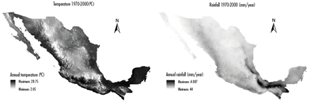
Source: Prepared by the authors based on data from WorldClim2.0 (Fick and Hijmans, 2017).
Figure 2 GIS climate databases
The average municipal altitude is calculated using the WorldClim 2.1 elevation raster. To calculate road density, the Red Nacional de Caminos (INEGI, 2014b), the Marco Geoestadístico Municipal 2014 and ArcGis tools are used to obtain the ratio between the total length of roads in a municipality compared with its entire area. The remaining control variables are taken from the ENA 2014.
Table 1 shows the descriptive statistics of the PU sample used to estimate the Ricardian model. On average, the net income per head of cattle is MXN$ 2,004.21The annual temperature ranges between 10.37 °C and 27.96 °C and the yearly rainfall between 6.55 mm/month and 337.30 mm/month. Variation in climate averages is a fundamental prerequisite for estimating the Ricardian model using cross-sectional data, so the sample temperature and rainfall ranges indicate sufficient variation in the climate to assess the Ricardian model. The average standard deviation for the period 1970-2000 in the municipalities where livestock activities are carried out, ranges from 0.63 to 8.00 °C and the coefficient for rainfall variation for the same period ranges from 63 to 133. The daytime temperature reflects the difference between the maximum daytime and minimum nighttime temperature, and in the PU sample of this paper, this value ranges from 8.15 to 20.28 °C. As in the case of long-term climate, there is a significant variation in the average altitude at which the PUs of the sample are located, between 1.65 and 3,225 meters above sea level (masl). Road density shows that, on average, in livestock production zones, there are 302 linear meters of roads for every km2.
Table 1 Descriptive statistics of the sample
| Variable | Obs. | Mean | SD | Mín. | Max. |
| Net income per PU ($*1 000/UP) | 28 337 | 404.4 | 5.676 | -111 766 | 650 000 |
| Net income per capita ($*1 000/cabeza) | 28 337 | 2.004 | 4.509 | -10.98 | 30.67 |
| Annual temperature (°C) | 28 337 | 20.21 | 4.363 | 10.37 | 27.96 |
| Annual rainfall (mm/mes) | 28 337 | 74.83 | 42.26 | 6.554 | 337.3 |
| The standard temperatura deviation (*100) | 28 337 | 293.6 | 141.5 | 62.74 | 799.5 |
| The rainfall coefficient variation | 28 337 | 92.09 | 19.93 | 42.25 | 132.7 |
| Variable | Obs. | Media | SD | Mín. | Máx. |
| Daytime temperature (°C) | 28 337 | 15.00 | 2.444 | 8.152 | 20.28 |
| Altitude (masl) | 28 337 | 1.237 | 898.1 | 1.649 | 3 225 |
| Road density (km/km2) | 28 337 | 0.302 | 0.258 | 0.00765 | 2.116 |
| Household size (members) | 28 337 | 3.736 | 2.059 | 1.00 | 32.00 |
| Age ot he producer (years) | 28 337 | 58.36 | 13.79 | 18.00 | 100.00 |
| Gender of the producer (1=male) | 28 337 | 0.907 | 0.290 | 0.00 | 1.00 |
| Education (years) | 28 337 | 3.349 | 2.002 | 0.00 | 8.00 |
| Indigenous (1=recoginized as indigenous) | 28 337 | 0.187 | 0.390 | 0.00 | 1.00 |
| PROGAN (1=the producer is benefitary) | 28 337 | 0.193 | 0.395 | 0.00 | 1.00 |
| Heads of cattle and swine (heads) | 28 337 | 106.4 | 838.3 | 1.00 | 50 000 |
| Head of cattle (head) | 28 337 | 65.82 | 422.7 | 0.00 | 50 000 |
| Head of swine (heads) | 28 337 | 40.56 | 710.7 | 0.00 | 44 000 |
Note: Obs: number of observation; Mean: average of the variable in the sample; SD; standard deviation; Min: minimum value in the sample; and Max: maximum value in the sample.
Source: Prepared by the authors with data from the National Agricultural Survey (INEGI, 2014a).
In addition to climate variables and location characteristics (altitude and road density), the Ricardian model includes a set of sociodemographic characteristics of the producer (household size, age, gender, education, ethnicity and subsidies). In the sample, the average age of the producers is 58 years old; men are in charge of 90.7% of the PUs, the average education level of the producers is 3.35 years (unfinished primary education) and 18.7% identify as being of indigenous origin. The PUs in the sample have, on average, 106 head of cattle and a median value of 20 head. In addition, a dichotomous variable is included to indicate whether the producer is a beneficiary of the PRO-GAN livestock subsidy program, with 19.2% of producers in the sample receiving such subsidies.
4. RESULTS
In this section, we present the results of the estimation of the Ricardian model defined in equation (4), the effects of marginal and non-marginal changes in temperature and rainfall on the net income per head of cattle defined in equations (5), (6) and (7). The following tests were performed to identify the best functional form of the Ricardian model. First, the distribution of the dependent variable shows negative values, which rules out the possibility of using the semilogarithmic functional form.22To solve this problem, the literature suggests shifting the distribution of the dependent variable to the right by adding a constant value, minimum value plus one, to each observation. However, this transformation has been widely criticized for influencing the results of the estimations that use a semilogarithmic functional form. Therefore, in this study, the dependent variable was used without any transformation, i.e., net income per head expressed in thousands of pesos.
Secondly, the relevance of including subsets of control variables in the Ricardian model was evaluated. The results of the F test23indicate that, together, the climate variables (F(5, 28314)=44.47, Prob > F=0.00), extreme weather variables (F(3, 28314)=107.28, Prob > F=0.00), PU attributes and sociodemographic characteristics of producers (F(10, 28314)=85.42, Prob > F=0.00) and fixed effects per region (F(4, 28314)=36.20, Prob > F=0.00) are statistically significant and should therefore be included in the Ricardian model. Likewise, the F-test suggests that, together, the squared terms of the climate variables (F(2, 28314)=36.99, Prob > F=0.00) and climate interactions (F(1, 28314)=38.15, Prob > F=0.00) are statistically significant. This confirms a non-linear relationship between climate and farmers' net income and that the marginal effects of temperature and rainfall depend on the current climate in each PU.
Table 2 presents the set of estimated parameters of the Ricardian model for all producers, cattle producers, swine producers, cattle and swine producers, large and small producers.24The estimates for different producer groups allow us to identify the diversity of effects of climate change on livestock production in Mexico. In the case of temperature, the coefficients associated with the squared term of the different types of PU are not statistically significant, except in the case of cattle, where an inverted U association with net income is found. In the case of rainfall, a U-type relationship is observed with respect to net income, except in swine production. It is also found that the coefficients associated with the interaction term between temperature and rainfall are, for the most part, statistically significant, suggesting that the marginal effect of a climate variable depends on the current level of the other variable, i.e., the impact of an additional degree of global warming does not affect a PU with 30 mm/month in the same way as a PU with 120 mm/month of rainfall and vice versa.
Table 2 Estimated parameters of the Ricardian model
| Variable | All | Cattle | Swine | Cattle and swine | Small | Large |
| Temperature | -0.1055 | 0.0628 | 0.0725 | -0.4045** | -0.0144 | -0.2089* |
| (0.0736) | (0.0962) | (0.0823) | (0.1687) | (0.0860) | (0.1234) | |
| Temperature ^2 | -0.0039 | -0.0104*** | -0.0027 | 0.0083 | -0.0030 | -0.0030 |
| (0.0024) | (0.0031) | (0.0027) | (0.0056) | (0.0029) | (0.0038) | |
| Rain | -0.0716*** | -0.0811*** | 0.0145** | -0.0510*** | -0.0194*** | -0.1091*** |
| (0.0064) | (0.0087) | (0.0063) | (0.0134) | (0.0072) | (0.0112) | |
| Rain^2 | 0.000076*** | 0.000059*** | -0.000007 | 0.000065*** | 0.000026* | 0.000095*** |
| (0.000011) | (0.000013) | (0.000015) | (0.000023) | (0.000015) | (0.000015) | |
| Temperature*Rain | 0.0019*** | 0.0024*** | -0.0004 | 0.0012* | 0.0004 | 0.0029*** |
| (0.0003) | (0.0004) | (0.0003) | (0.0007) | (0.0004) | (0.0005) | |
| SD of temperature*100 | 0.0029*** | 0.0015** | -0.0017** | 0.0063*** | 0.0012* | 0.0018*** |
| (0.0005) | (0.0006) | (0.0008) | (0.0012) | (0.0007) | (0.0007) | |
| Coef. Rainfall var. 0.0270*** | 0.0235*** | 0.0059** | 0.0289*** | 0.0100*** | 0.0177*** | |
| (0.0017) | (0.0021) | (0.0026) | (0.0034) | (0.0023) | (0.0024) | |
| Daytime 0.0768*** | 0.1404*** | 0.0148 | -0.1128** | 0.0246 | 0.0503 | |
| (0.0242) | (0.0315) | (0.0268) | (0.0496) | (0.0281) | (0.0378) | |
| Altitude -0.0009*** | -0.0011*** | -0.0003 | 0.0001 | -0.0005* | -0.0006* | |
| (0.0002) | (0.0002) | (0.0003) | (0.0004) | (0.0002) | (0.0003) | |
| Road Density 2.4610*** | 3.1876*** | 0.0242 | 1.5097*** | 0.8819*** | 4.9162*** | |
| (0.1710) | (0.2242) | (0.1802) | (0.3578) | (0.1794) | (0.2855) | |
| Household size 0.0190 | 0.0611*** | -0.0010 | 0.1025*** | 0.0305* | 0.0367* | |
| (0.0140) | (0.0187) | (0.0146) | (0.0279) | (0.0160) | (0.0217) | |
| Age -0.0090*** | -0.0143*** | -0.0025 | -0.0066 | -0.0091*** | -0.0123*** | |
| (0.0020) | (0.0025) | (0.0025) | (0.0044) | (0.0025) | (0.0030) | |
| Man 0.8377*** | 0.7690*** | 0.2579*** | 0.3943** | 0.3871*** | 0.6067*** | |
| (0.0739) | (0.0983) | (0.0875) | (0.1577) | (0.0823) | (0.1214) | |
| Education 0.0989*** | 0.1056*** | -0.0046 | 0.0805*** | 0.0188 | 0.0890*** | |
| (0.0131) | (0.0165) | (0.0176) | (0.0281) | (0.0157) | (0.0196) | |
| Indigenous -0.7972*** | -0.7796*** | 0.1085 | -0.5145*** | -0.1621** | -0.5210*** | |
| (0.0621) | (0.0830) | (0.0754) | (0.1282) | (0.0737) | (0.0966) | |
| PROGAN 0.6654*** | 0.2996*** | 0.3437 | 0.8110*** | 0.1392 | 0.0663 | |
| (0.0547) | (0.0648) | (0.2480) | (0.1193) | (0.1100) | (0.0675) | |
| Variable | All | Cattle | Swine | Cattle and swine | Small | Large |
| Heads | 0.0006*** | 0.0026*** | 0.0003*** | 0.0001 | 0.6804*** | 0.0002** |
| (0.0001) | (0.0003) | (0.0001) | (0.0001) | (0.0205) | (0.0001) | |
| Heads^2 | -0.00000002*** | -0.00000005*** | -0.00000001*** | -0.000000002 | -0.0228*** | -0.00000001 |
| (0.000000005) | (0.00000001) | (0.000000002) | (0.00000000) | (0.0010) | (0.000000004) | |
| Central region | -0.6386*** | -0.6924*** | -0.1226 | -0.4054 | 0.1325 | -0.5399** |
| (0.1276) | (0.1737) | (0.1397) | (0.2563) | (0.1466) | (0.2313) | |
| Midwest region | -0.7760*** | -0.8849*** | 0.3575** | -0.8738*** | -0.6299*** | -1.1422*** |
| (0.0933) | (0.1153) | (0.1673) | (0.2215) | (0.1330) | (0.1322) | |
| Northeast region -1.5660*** | -1.9132*** | 0.5394** | -1.4207*** | -1.0950*** | -2.0584*** | |
| (0.1306) | (0.1598) | (0.2567) | (0.2725) | (0.1859) | (0.1798) | |
| Northwest region -1.5480*** | -1.8099*** | 1.1221 | -1.7838*** | -0.3486 | -1.9721*** | |
| (0.1784) | (0.2097) | (0.7117) | (0.4162) | (0.2893) | (0.2308) | |
| Southeast region - (ommited) | - | - | - | - | - | |
| Constant | 3.4558*** | 3.4305*** | -1.2954 | 4.2837* | -1.1165 | 8.4748*** |
| (1.0273) | (1.3108) | (1.1878) | (2.1946) | (1.3000) | (1.5975) | |
| Remarks | 28 337 | 20 747 | 3 530 | 4 060 | 14 464 | 13 873 |
| R-squared | 0.065 | 0.089 | 0.039 | 0.063 | 0.143 | 0.115 |
Note: the dependant variable is net income per head expressed in thousands of pesos. Estiamates include region-fixed effects. Robust standard errors in parentheses. *** p<0.01; ** p<0.05; * p<0.1.
Source: Prepared by the authors with data from the National Agricultural Survery (INEGI, 2014a).
Contrary to initial expectations, more significant long-term climate variation is usually associated with higher net income. In the case of the standard deviation of temperature, when this variation is more significant, net income is higher, except for specialized swine producers, where temperature stress may generate greater susceptibility to disease. In the case of the variation coefficient of rainfall and daytime temperature, the same relationship is observed in most of the samples. Since it is assumed that producers have adapted to the current climate conditions of the place where they are located, this result may occur due to market conditions. Thus, it was argued that product prices are higher in places with more significant climate variation, and therefore, net income may be higher.
The coefficients associated with altitude are generally negative and statistically significant, suggesting that PUs located at high altitudes tend to have lower net income per head of cattle. Taking the sample of all PUs, an additional 100 MASL is associated with an MXN$90 lower net income. In the case of swine, this association is not statistically significant. An increase in road density is associated with higher net income levels. Road density is included in the Ricardian model to incorporate the PUs' connectivity to markets. The results show that investment in overland roads can significantly impact the net income of livestock farmers. This is because being better connected to the market allows farmers to purchase better quality inputs at a lower cost by avoiding transportation costs and selling products more quickly than PUs located in remote areas.
Previous studies use household size as a control for family labor costs, which are regularly underreported in available surveys. The results indicate that household size has a positive and statistically significant relationship with net income, in line with the findings of Kabubo-Mariara (2009). In accordance with initial expectations, producer age is inversely associated with the amount of net income, i.e., younger producers tend to have higher net incomes; men have higher net incomes than women; an additional year of education is associated with higher net income levels, i.e., the income for an additional year of education is, on average, MXN$99 per head of cattle. Meanwhile, producers who identify themselves as being indigenous have net incomes per head MXN$797 lower than other livestock producers. Based on the foregoing, it could be inferred that older, female, poorly educated farmers and members of Indigenous communities are more vulnerable to climate change.
There is an inverted U relationship between the number of head of cattle and net income per head. This suggests a tipping point where the marginal contribution of an additional animal to net income becomes negative. The coefficient associated with the PROGAN subsidy indicator suggests that, on average, its beneficiaries have higher net incomes than producers who do not receive such transfers. This could indicate the regressivity of the program, i.e., the transfers are directed to producers with higher profits. Finally, the Ricardian model includes dichotomous variables indicating the region in which the PU is located to capture structural differences between one area and another, determining the level of net income per head in the sample.
Using the estimated parameters from Table 2 and the mean temperature and rainfall values for each sample, Table 3 presents the marginal effects of the climate variables on net revenue per head of cattle in the corresponding samples. On average, one additional degree of temperature is expected to decrease net income per head by -MXN$118.5 (5.89% of current value). This effect ranges from -MXN$98.9 and -MXN$180.7 per head, depending on the type of producer. In the case of specialized swine producers and non-specialized producers (swine and cattle), the marginal effect evaluated in the mean values is not statistically significant. Swine in Mexico are generally housed, so producers can more easily deal with a rise in temperature than those producing free-grazing cattle.
Table 3 Marginal effects of temperature and rainfall
| Variable | All | Cattle | Swine | Cattle and swine | Small | Large |
| Temperature (°C) | -0.1185*** | -0.1807*** | -0.0713 | 0.0035 | -0.0989** | -0.1200** |
| (0.0372) | (0.0459) | (0.0454) | (0.0730) | (0.0459) | (0.0546) | |
| Rainfall(mm/month) | -0.0211*** | -0.0223*** | 0.0046** | -0.0187*** | -0.0071*** | -0.0346*** |
| (0.0015) | (0.0018) | (0.0021) | (0.0034) | (0.0020) | (0.0022) | |
| Remarks | 28 337 | 20 747 | 3 530 | 4 060 | 14 464 | 13 873 |
Note: Standard error in brackets; *** p<0.01; ** p<0.05; * <0.1.
Source: Prepared by the authors with data from the National Agricultural Survey (INEGI, 2014a).
When evaluating equation (6) in the mean values, an additional mm/month would represent a decrease in net income per head of -MXN$21.1 pesos if all PUs in the sample are considered. This value is between -MXN$34.6 and MXN$4.6, where the only ones benefiting from the marginal change in rainfall are producers specialized in swine production.
Fick and Hijmans (2017) use a set of GCMs to construct raster databases with estimates for the future global climate for the periods 2041-2060 and 2081-2100. Using the municipal average of the values generated by the GCM ACCESS-ESM1-522525and the coefficients in Table 2, the current climate is replaced with the future climate and the change in net income per head is calculated in each of the PUs in the sample. Table 4 shows the average values of current and future temperature, rainfall and net income per head for the periods 2041-2060 and 2081-2100 pursuant to the SSP126 and SSP5852626scenarios (see IPCC, 2022 for the full description of the SSP126 and SSP585 scenarios). The estimated parameters and corresponding values for each of the samples for which the Ricardian models are estimated are shown in table 2. The minimum and maximum values for each distribution variable are shown in square brackets.
Table 4 Impacts of climate change on the net income of livestock farmers in Mexico
| ACCESS-ESM1-5 | |||||||
| Variable | 1970-2000 | 2041-2060 | 2081-2100 | Variable | 1970-2000 | 2041-2060 | 2081-2100 |
| Current | SSP126 | SSP585 | SSP126 | SSP585 | |||
| All PUs | |||||||
| Temperature (°C) | 20.21 [10.37-27.96] | 22.31 [12.54-30.50] | 23.05 [13.22-31.41] | 22.39 [12.62-30.81] | 25.46 [15.53-34.43] | ||
| Rainfall (mm/mo) | 74.83 [6.55-337.30] | 73.84 [6.86-332.40] | 68.31 [6.80-302.10] | 73.57 [6.85-325.70] | 57.81 [7.22-255.40] | ||
| Net income/head ($*1 000) | 2.004 [-10.98-30.67] | 1.735 [-11.25-30.42] | 1.666 [-11.32-30.44] | 1.715 [-11.25-30.41] | 1.326 [-11.68-30.28] | ||
| Net income/head (%) | -13.42 | -16.87 | -14.42 | -33.83 | |||
| Cattle | |||||||
| Temperature (°C) | 20.45 [10.48-27.96] | 22.55 [12.65-30.50] | 23.30 [13.33-31.41] | 22.63 [12.73-30.81] | 25.70 [15.65-34.43] | ||
| Rainfall (mm/mo) | 74.35 [6.55-337.30] | 73.47 [6.86-332.40] | 68.01 [6.80-302.10] | 73.24 [6.85-325.70] | 57.72 [7.22-255.40] | ||
| Net income/head ($*1 000) | 2.490 [-10.98-30.67] | 2.060 [-11.52-30.43] | 1.915 [-11.73-30.47] | 2.031 [-11.54-30.41] | 1.262 [-12.53-30.26] | ||
| Net income/head (%) | -17.27 | -23.09 | -18.43 | -49.32 | |||
| Swine | |||||||
| Temperature (°C) | 19.63 [10.37-27.89] | 21.73 [12.54-30.00] | 22.47 [13.22-30.78] | 21.81 [12.62-30.26] | 24.86 [15.53-33.31] | ||
| Rainfall (mm/mo) | 81.97 [9.24-333.90] | 80.35 [9.68-317.50] | 73.93 [9.55-291.30] | 79.80 [9.68-311.70] | 61.67 [9.98-239.50] | ||
| Net income/head ($*1 000) | -0.353 [-10.70-28.33] | -0.517 [-10.83-28.19] | -0.593[-10.90-28.13] | -0.525 [-10.83-28.20] | -0.826 [-11.11-27.91] | ||
| Net income/head (%) | -46.46 | -67.99 | -48.73 | -133.99 | |||
| Cattle and swine | |||||||
| Temperature (°C) | 19.49 [10.48-27.51] | 21.58 [12.65-30.03] | 22.33 [13.33-30.98] | 21.65 [12.73-30.34] | 24.75 [15.65-34.03] | ||
| Rainfall (mm/mo) | 71.07 [9.24-333.90] | 70.08 [9.68-317.50] | 64.97 [9.55-291.30] | 69.87 [9.68-311.70] | 54.89 [9.98-239.50] | ||
| Net income/head ($*1 000) | 1.568 [-10.80-29.91] | 1.612 [-11.11-29.82] | 1.689 [-11.13-29.89] | 1.612 [-11.14-29.81] | 1.928 [-11.21-30.08] | ||
| Net income/head (%) | 2.81 | 7.72 | 2.81 | 22.96 | |||
| Small producers | |||||||
| Temperature (°C) | 19.60 [10.37-27.96] | 21.71 [12.54-30.50] | 22.45 [13.22-31.41] | 21.79 [12.62-30.81] | 24.86 [15.53-34.43] | ||
| Rainfall (mm/mo) | 76.09 [6.55-333.90] | 74.93 [6.86-317.50] | 69.31 [6.80-291.30] | 74.63 [6.85-311.70] | 58.39 [7.22-239.50] | ||
| Net income/head ($*1 000) | 1.059 [-10.98-30.67] | 0.840 [-11.24-30.49] | 0.774 [-11.30-30.47] | 0.828 [-11.24-30.48] | 0.508 [-11.58-30.32] | ||
| Net income/head (%) | -20.68 | -26.91 | -21.81 | -52.03 | |||
| Large producers | |||||||
| Temperature (°C) | 20.85 [10.48-27.96] | 22.94 [12.64-30.50] | 23.69 [13.29-31.41] | 23.02 [12.71-30.81] | 26.09 [15.57-34.43] | ||
| Rainfall (mm/mo) | 73.52 [9.24-337.30] | 72.70 [9.68-332.40] | 67.27 [9.55-302.10] | 72.47 [9.68-325.70] | 57.20 [9.98-255.40] | ||
| Net income/head ($*1 000) | 2.989 [-10.89-30.52] | 2.719 [-11.34-30.21] | 2.685 [-11.39-30.24] | 2.697 [-11.40-30.17] | 2.392 [-11.70-30.13] | ||
| Net income/head (%) | -9.03 | -10.17 | -9.77 | -19.97 | |||
Note: the values in square brackets indicate the range of variation [minimum-maximum] of the corresponding variable.
Source: Prepared by the authors based on estimates of the Ricardian model; Fick and Hijmans (2017).
When considering the sample of all the PUs contained in the 2014 ENA, it can be observed that the temperature of the areas where they are located could increase between 2.10 °C and 2.84 °C between 2041 and 2060 and between 2.18 °C and 5.25 °C in 2081-2100 depending on the trajectories of GHG accumulation in the atmosphere. In addition, rainfall could decrease between -0.99 mm/month (1.32%) and -6.52 mm/month (8.71%) for the period 2041-2060 and between -1.26 and -1.26 mm/month (8.71%) for the period 2041-2060 mm/month (1.68%) and -17.02 mm/month (22.74%) for the period 2081-2100. Thus, the ACCESS-ESM1-5 GCM estimates, on average, a drier and warmer future for the areas where cattle and swine are produced in Mexico. By substituting the current climate with the future climate in each of the PUs, as indicated in equation (7), the results suggest that net income per head could decrease between -13.42 and -16.87% for the period 2041-2060 and between -14.42 and -33.83% concerning its current level.
The combination of increased temperature and decreased rainfall will result in significant losses for producers specializing in swine production. Based on the set of climate change scenarios, the losses of these producers could amount to 134% of the current average net income per head, if the SSP585 scenario is considered for the period 2081-2100. On the other hand, producers who do not specialize in a single species could benefit from such climate changes. The results in Table 4 show that the net income per head of mixed PUs could increase at the average annual growth rate for the 2041-2060 period between 2.81% and 7.72% and even increase between 2.81% and 22.96% for the 2081-2100 period. This result is consistent with several studies which argue that production diversification significantly reduces vulnerability to climate change (Mendelsohn and Dinar, 2009).
Considering the PU’s size, Table 4 shows that small farmers are more vulnerable to climate change than large farmers. For the period 2041-2060, the first group could face losses of between -20.7 and -26.9% of their current net income per head, while for the second group, such decreases would range between -9.0 and -26.9% of their current net income per head -10.2%. Likewise, by 2081-2100, small producers could face losses of up to -52% and large producers of up to -20%.
The results coincide with the estimates of Mendelsohn et al. (2010) and Galindo et al. (2015) regarding the magnitude of losses that climate change may cause to producers in the primary sector. Mendelsohn et al. (2010) estimate that by 2100, the value of agricultural land per hectare may decrease by -42 to -54% from the current value due to climate change. Galindo et al. (2015) estimate that by 2100 producers will face losses of between -18.6 and -36.4% of their net income per hectare compared with current levels. When analyzing the livestock sector, it was found that, based on 2100, the change in net income per head of cattle could range from -14.4% to -33.8% by 2100. Undoubtedly, changes in the climate could generate a significant loss of income for the people who depend on the primary sector in Mexico, as well as a considerable reduction in the food supply. Therefore, economic policies implemented in the coming years must focus on reducing the sector’s vulnerability.
The following economic policy recommendations can be derived from this research: first of all, given that older, female, indigenous, less educated and small producers are more vulnerable to changes in climate conditions, policymakers should focus their efforts on reducing the gaps between these groups and their counterparts. Secondly, species diversification within the PU should be promoted to reduce vulnerability to climate change. To this end, economic policy must support producers with investments in infrastructure that allow for such diversification, especially small producers who often do not have sufficient savings or sources of credit to make this type of investment, for example, new paddocks, feedlots, grazing areas, warehouses, among others.
In addition to the economic policy recommendations, the following is established based on this paper: first of all, despite efforts to calculate livestock income (net income) per hectare, we need more information collected by the ENA 2014 to allow us to do so. This problem persists in the literature using the Ricardian method in the livestock sector, especially for free-grazing cattle where the area needed for production needs to be clarified (Kabubo-Mariara, 2009). In Mexico, there are state-level pasture coefficients and area standards for livestock grazing. When these parameters were used in this research, the results were inconsistent due to the assumption of similarity in the pasture area within the same state and between productive structures of different PUs for stabled cattle. Secondly, the results of this research consider the direct effect of climate on net income per head; however, it is important to consider the indirect effect that could be generated by the impacts of climate change on the availability of feed for livestock. This second consideration provides a line of future research to be addressed.
It is important to note that the results of previous studies and this paper are based on the principle of Ceteris paribus, i.e., the estimated changes result from maintaining all other factors affecting land rent or net income constant. Therefore, changes in other variables may influence the results. For example, if there is a significant development of the road network, this could reduce estimated losses since the Ricardian model suggests that when road density increases, PUs tend to have higher levels of net income per head of cattle.
5. CONCLUSIONS
This article aims to identify the impacts of climate change on Mexico's livestock production. For this purpose, a set of Ricardian models is estimated using financial information from 28,337 PU of cattle and swine reported in the ENA 2014. The Ricardian models relate net income per head of cattle to climate variables, PU characteristics, socio-demographic characteristics of producers and structural factors on a regional level using linear regression. Using different groups of producers, it was possible to identify the diversity of marginal and non-marginal impacts of climate change on livestock. The main findings suggest that, on average, changes in net income per head of cattle could be between -13.42 and -16.87% in the period 2041-2060, and between -14.42 and -33.83% in the period 2081-2100, compared with current levels due to climate change. It is also found that producers specializing in a single livestock species and small producers are more vulnerable to climate change.
The following economic policy recommendations can be derived from the results of this research: i) reduce areas of vulnerability to climate change by designing and implementing programs that focus on the elderly, women, indigenous people, less educated and small producers; and ii) promote the diversification of livestock activities through training or access to credit and/or financing so that producers can make investments, which allow them to produce more than one species, e.g., new paddocks, feedlots, grazing areas, warehouses, among others. In terms of research, it is suggested to continue with the following: i) identify the indirect impact that climate change could have on net livestock income through the availability of feed for livestock under different climate change scenarios, and ii) explicitly demonstrate in a Ricardian model the adaptation strategies that producers could implement to reduce their vulnerability to climate change, e.g. the ability to place free-grazing livestock in stables.
When interpreting the results, the reader should consider the following points: first, the ENA 2014 collects information from the agricultural sector for one agrarian year, so some income or costs may not be reported correctly. In the case of livestock, income from the sale of fattening animals or breeding stock may not be reported in the year in which producers were interviewed. Furthermore, long-term investment or depreciation costs may not be reported in the survey year, e.g., the purchase of cattle or depreciation of the dairy herd. It is considered that this measurement error is found in the residuals of the Ricardian model estimation and is random and, therefore, does not influence the estimated parameter values. Secondly, the net income per head does not include the deduction of the cost of labor, the cost of manufactured capital and the cost of natural capital due to issues regarding availability of information. Therefore, net income should be considered a measure of income for the previous three factors.
ACKNOWLEDGMENTS
Research carried out thanks to the UNAM-PAPIIT-IA303221 Program Impact of climate change on food production in Mexico. The authors are extremely grateful for the comments of those who reviewed earlier versions of this article and contributed to improving the paper. We are also thankful for the support from the microdata laboratory and the department responsible for the National Agricultural Survey at the National Institute for Statistics and Geography (INEGI).
REFERENCES
Banco de México (BM) (2022). Tipos de cambio y resultados históricos de las subastas. Base de datos de Banco de México: https://www.banxico.org.mx/SieInternet/consultarDirectorioInternetAction.do?sector=6&accion=cons ultarCuadro&idCuadro=CF86&locale=es [ Links ]
Basurto-Hernández, S. (2019). Essays on climate change, agriculture and production efficiency (Doctoral dissertation, University of Birmingham). https://etheses.bham.ac.uk/id/eprint/9254/ [ Links ]
Batsuuri, T. y Wang, J. (2017). The impacts of climate change on Nomadic livestock husbandry in Mongolia. Climate Change Economics, 8(03). https://doi.org/10.1142/s2010007817400036 [ Links ]
Bozzola, M., Massetti, E., Mendelsohn, R. y Capitanio, F. (2018). A Ricardian analysis of the impact of climate change on Italian agriculture. European Review of Agricultural Economics, 45(1). https://doi.org/10.2139/ ssrn.2983021 [ Links ]
Fick, S. E. y Hijmans, R. J. (2017). WorldClim 2: new 1-km spatial resolution climate surfaces for global land areas. International journal of climatology, 37(12). https://doi.org/10.1002/joc.5086 [ Links ]
Food and Agriculture Organization of the United Nations (2022). FAOSTAT statistical database. FAO. [ Links ]
Galindo, L. M., Reyes, O. y Alatorre, J. E. E. (2015). Climate change, irrigation and agricultural activities in Mexico: A Ricardian analysis with panel data. Journal of Development and Agricultural Economics, 7(7). https://doi. org/10.5897/jdae2015.0650 [ Links ]
Gebreegziabher, Z., Mekonnen, A., Deribe, R., Abera, S. y Kassahun, M. M. (2013). Crop-ivestock inter-linkages and climate change implications for Ethiopia’s agriculture: A Ricardian approach. Resources For the Future. [ Links ]
Instituto Nacional de Estadística y Geografía (INEGI) (2014a). Encuesta Nacional Agropecuaria 2014. Microdatos: https://www.inegi.org.mx/programas/ena/2014/ [ Links ]
______ (INEGI) (2014b). Red Nacional de Caminos RNC. 2014. https://www.inegi.org.mx/app/biblioteca/ficha.html?upc=702825278724 [ Links ]
Kabubo-Mariara, J. (2009). Global warming and livestock husbandry in Kenya: Impacts and adaptations. Ecological Economics, 68(7). https://doi. org/10.1016/j.ecolecon.2009.03.002 [ Links ]
Mendelsohn, R., Nordhaus, W. D. y Shaw, D. (1994). The impact of global warming on agriculture: a Ricardian analysis. The American Economic Review, 84(4). http://www.jstor.org/stable/2118029 [ Links ]
Mendelsohn, R. y Seo, S. N. (2007). A structural Ricardian analysis of climate change impacts and adaptations in South American farms. Policy Research Working Paper (No. 4161). [ Links ]
______ y Dinar, A. (2009). Climate change and agriculture: an economic analysis of global impacts, adaptation and distributional effects. Edward Elgar Pu- blishing. [ Links ]
_______, Arellano-Gonzalez, J. y Christensen, P. (2010). A Ricardian analysis of Mexican farms. Environment and Development Economics, 15(2). https://doi.org/10.1017/s1355770x09990143 . [ Links ]
Organisation for Economic Co-operation and Development (2021). OECD- FAO Agricultural Outlook. Edition 2021: https://data.OECD.org/agroutput/ meat-consumption.htm [ Links ]
Panel Intergubernamental de expertos sobre el Cambio Climático (IPCC) (2021). Summary for Policymakers. En V. Masson-Delmotte, P. Zhai, A. Pirani, S. L. Connors, C. Péan, S. Berger, N. Caud, Y. Chen, L. Goldfarb, M. I. Gomis, M. Huang, K. Leitzell, E. Lonnoy, J. B. R. Matthews, T. K. Maycock, T. Waterfield, O. Yelekçi, R. Yu y B. Zhou (eds.). Climate change 2021: The physical science basis. Contribution of working group I to the sixth assessment report of the intergovernmental panel on climate change. Cambridge University Press. In Press. [ Links ]
_______ (2022). Climate change 2022: Impacts, adaptation, and vulnerability. Contribution of working group II to the sixth assessment report of the intergovernmental panel on climate change. Cambridge University Press. [En prensa]. [ Links ]
Secretaría de Agricultura y Desarrollo Rural (SADER) (2021). Sistema de Información Agroalimentaria de Consulta-SIACoN. Edición 2021. https://www.gob.mx/siap/documentos/siacon-ng-161430 [ Links ]
Seo, S. N. (2016). Modeling farmer adaptations to climate change in South America: a micro-behavioral economic perspective. Environmental and Ecological Statistics, 23(1). https://doi.org/10.1007/s10651-015-0320-0. [ Links ]
_______ y Mendelsohn, R. O. (2007a). Climate change impacts on animal husbandry in Africa: A Ricardian analysis. World Bank Policy Research Working Paper, (4261). https://papers.ssrn.com/sol3/papers.cfm?abstract_ id=996167 [ Links ]
_______ y Mendelsohn, R. O. (2007b). The impact of climate change on lives- tock management in Africa: a structural Ricardian analysis, vol. 4279. World Bank Publications. http://hdl.handle.net/10986/7463 [ Links ]
_______ y Mendelsohn, R. O. (2008a). Animal husbandry in Africa: climate change impacts and adaptations. African Journal of Agricultural and Resource Economics, 2(311-2016-5520). https://ageconsearch.umn.edu/re cord/56968/ [ Links ]
_______ y Mendelsohn, R. O. (2008b). A structural Ricardian analysis of climate change impacts and adaptations in African agriculture, vol. 4603. World Bank Publications. http://hdl.handle.net/10986/6770 [ Links ]
_______ y Mendelsohn, R. O. (2008c). Climate change impacts on Latin American farmland values: the role of farm type. Revista de Economia e Agronegocio/Brazilian Review of Economics and Agribusiness, 6(822-2016- 54194). https://ageconsearch.umn.edu/record/53872 [ Links ]
_______ y Mendelsohn, R. O. (2008d). Measuring impacts and adaptations to climate change: a structural Ricardian model of African livestock management 1. Agricultural economics, 38(2). https://doi.org/10.1111/j.1574-0862.2007.00289.x [ Links ]
Tibesigwa, B., Visser, M. y Turpie, J. (2017). Climate change and South Africa’s commercial farms: an assessment of impacts on specialised horticulture, crop, livestock and mixed farming systems. Environment, Development and Sustainability, 19(2). https://doi.org/10.1007/s10668-015-9755-6 [ Links ]
Organización de las Naciones Unidas (ONU) (2019). World Population Prospects 2019, Online Edition. Rev. 1. [ Links ]
Van Passel, S., Massetti, E. y Mendelsohn, R. (2017). A Ricardian analysis of the impact of climate change on European agriculture. Environmental and Resource Economics, 67(4). https://doi.org/10.2139/ssrn.2463134 [ Links ]
6A population of 128.93 million people is estimated for 2020 (UN, 2019). A decrease in Mexico's population is also estimated from the year 2063 onwards (UN, 2019).
7The average of the climate projections from the ACCESS-ESM1-5 model in Fick and Hijmans is used (2017).
8 In the case of temperature and rainfall, the dependent variable can be land value per hectare, net income per PU or net income over total livestock value.
10 It is assumed that the prices of food, labor and capital do not vary by species or between PU, i.e., producers are price takers of these inputs.
11 The reduced form is a functional form that takes into consideration those inputs that are exogenous; therefore, the set of endogenous inputs/variables (Gi, Fi, Li, Ki) can be omitted.
14 The summation starts at q=6 to continue with the parameter numbering of the Ricardian model in an abbreviated form.
15 There are the ENA 2012, 2014, 2017 and 2019 surveys, however, the only one that has information on production costs and total income in the entire sample is the ENA 2014, which is why only that one was used.
16 Total revenues comprise revenues from the sale of milk, cattle and pigs in production between 2013-2014. The ENA 2014 does not provide sufficient information to estimate net income from poultry, sheep or goats.
17 Total expenditure comprises the amount spent on feed, food supplements, medicines, vaccines, surgeries, medical care and genetic improvement of the animals.
19 Ricardian models regularly use net income per hectare, or unit of land; however, in livestock farming it is not possible to identify the area of livestock production, especially in countries with common lands (or ejidos, as in the case of Mexico) where free grazing practices are carried out. Therefore, existing literature suggests considering net income per head of cattle.
20 The objective of PROGAN is to contribute to increasing productivity in the PU through investment in the livestock sector. Support is granted to ejido owners, settlers and communal farmers, small landowners, and civil or mercantile companies established in accordance with Mexican law, owners of or persons with the right to use grazing land dedicated to extensive livestock raising, through the use of native vegetation or pastures, who are registered in the National Livestock Register (PGN). In 2014, program beneficiaries received MXN$1,800 per bovine calf of reproductive age distributed as follows: MXN$300 for the first year, MXN$400 for the second year, MXN$500 for the third year and MXN$600 for the fourth year. In the case of pigs, the amount was MXN$117 per pig.
23 The null hypothesis of the F-test indicates that the estimated parameters for the corresponding set of control variables are not statistically significant at the 5% significance level.
24 To differentiate between large and small producers, the median was taken of the distribution of the number of head of cattle owned by the PUs in the sample. Small producers have 1 to 20 head of cattle and large producers have more than 20 head of cattle.
25 A wide variety of simulations of future climate have been used in existing Ricardian studies. This paper uses the future climate simulations of the ACCESS-ESM1-5 GCM because it offers a wide range of possible scenarios for climate change in Mexico, i.e., the impacts of minor and drastic changes in climate on producers' net incomes can be assessed.
27For presentation purposes, SSP 126 and 585 were selected, which capture extreme trajectories of greenhouse gas emissions and, therefore, extremes in temperature and rainfall changes. Therefore, the range of estimates presented in this research work encompasses the results obtained by using intermediate scenarios: SSP 245 and 370. Although there are climate projections for the periods 2021-2040 and 2061-2080, results are only presented for the periods 2041-2060 and 2081-2100 to show mid- and end-of-century estimates and improve the presentation of results.
Received: April 12, 2022; Accepted: October 12, 2022
 Este es un artículo publicado en acceso abierto bajo una licencia Creative Commons
