


 nova página do texto(beta)
 Inglês (pdf)
 Artigo em XML
 Referências do artigo
 Enviar este artigo por email
 Citado por SciELO
  Similares em
SciELO
Similares em
SciELO 
 Permalink
Introduction
Tinnitus refers to listening to a sound but without an external source. Being a public health problem with a prevalence from 4 % to 37 % in the worldwide population and a frequent heterogeneous auditory condition with no standard and effective treatment1. It is well known that tinnitus tends to mostly affect elderly population, possibly due to the hearing loss (HL) as result of aging. Youthful population who suffers from tinnitus has been, however, significantly increased recently because of frequent exposure to recreational and occupational sounds without protective standards2. The diversity of tinnitus suffering is due to instability in how it is perceived, how it is generated, to psychological problems and to the efficacy of treatment3. Regarding the perception by humans, the buzz can be heard by all people, who have some kind of hearing loss as well as those who do not; can be heard in one ear in both ears; and pure tones, high-frequency whistles and cicada noises can be perceived4. As for the factors that cause tinnitus, the origin cannot be determined in most people. Recently it was considered a neurological problem5. The history of tinnitus is complex, as it is the result of a cortical reset at the tonotopic level due to neural desynchronization in the auditory cortex and limbic system6. The origin is due to many factors, including acoustic trauma, ototoxicity, multifactorial corticopathy, and vascular or tumor factors. Regarding the psychological effects, patients suffering from tinnitus frequently experience anxiety, depression, anguish, fear, anger and suicide. However, so far there are some treatments, including medication, surgery and hearing aids, psychological counseling and cognitive behavioral therapy (CBT), herbal treatments, acupuncture, acoustic therapies and serious auditory training games7. Still, the response to treatment is in most cases uncertain. The accurate identification and characterization of tinnitus is still a controversial issue. So far, three types of clinical methods are applied to diagnose tinnitus: 1) psychometric, 2) audiology, and 3) electrophysiological testing. For psychometric testing, there exists many questionnaires to monitor tinnitus status, evolution and side effects. Some of the most commonly applied questionnaires for monitoring tinnitus includes tinnitus handicap inventory8, hospital anxiety and depression scale9, tinnitus reaction questionnaire10, insomnia severity index11, quality of life inventory12, clinical global impression-improvement13, tinnitus acceptance questionnaire14, Beck depression inventory15, tinnitus functional index16, health utilities index score17, tinnitus sample case history questionnaire18, tinnitus catastrophizing scale19, perceived stress questionnaire20, and hyperacusis questionnaire21. In addition, several authors prefer make their own questionnaires to evaluate the condition for example22 who monitored patient reported outcomes and self-reporting of treatment, and23 who applied several questionnaires to evaluate tinnitus severity. For audiology testing, a detailed assessment of the auditory system is recommended, or even mandatory, to detect and characterize tinnitus. Most of the applied audiology methods includes otoacoustic emissions, transient evoked otoacoustic emission, high frequency audiograms (125Hz - 16kHz), speech in noise test, and threshold equalizing noise24. For electrophysiological testing, electrocochleography (ECochG) and electroencephalography (EEG) techniques are usually undertaken as well. In addition, other neuroimaging techniques have been used such as functional magnetic resonance imaging, magnetoencephalography (MEG), and near infrared spectroscopy (NIRS)2. As can be seen, tinnitus detection and characterization require a carefully elaborated diagnosis mainly owing to its heterogeneity nature. An inappropriate diagnosis often leads to inefficient treatment. Therefore, the present investigation aims to find EEG features in time and frequency domain that could distinguish between healthy and tinnitus sufferers with HL. In addition, this investigation pursues to give an insight into the group of tinnitus sufferers to search tendencies of those EEG features related to the HL of the sufferers. The latter through statistical analysis that demonstrate which is a promising neuromarker and stabilizing the differences between them. As a result, neuromarkers to identify tinnitus, along with the associated HL, can be proposed for diagnosis and monitoring of this auditive condition.
Diagnostic Approach to Tinnitus
It can be inferred that the diagnosis of tinnitus is complex, in terms of distinguishing between causal factors, types and location of the tinnitus perception. The patient perception of the noise that it is experienced due to tinnitus is classified as: tonal, pulsatile, filtered noise and musical25. Tonal tinnitus is perceived continuously by superimposed sounds with defined frequencies, the intensity is diverse, it is associated with subjective tinnitus. Instead, the pulsatile is a sound that can be in sync with the patient heartbeat, being an objective tinnitus. On the other hand, the filtered noise is a continuous broad band noise filtered at tinnitus frequency of the patient. Finally, musical tinnitus is characterized by the perception of simple or complex melodies that are referred to as musical instruments, sometimes accompanied by a singing voice, it is also often called musical ear syndrome26. Because the level of signal processing in patients with tinnitus implies a deficient procedure in the ascending auditory pathways and the cerebral cortex, there is currently no effective method for diagnosing tinnitus, much less an effective cure. There is a clinical follow-up of this complex symptom, being the task of audiologists and otolaryngologists to carry out an evaluation of the patient to achieve the most accurate diagnosis. Such as an otological test of the neck, a test of temporomandibular function, and a detailed evaluation of the patient history. For example, in audiometry, determining air conduction and bone conduction threshold levels helps differentiate between two types of HL: sensorineural hearing loss and conductive hearing loss. In addition, high-frequency audiometry (at least up to 16 kHz) is recommended27. The tinnitus pitch test (acufenometry) includes a set of audiological techniques to characterize the tinnitus frequency based on pure tones. Tinnitus is highly dependent on the ability of patients to identify the sound of their tinnitus. It also depends on the experience of the doctor. In the case of unilateral tinnitus, the test is easier as it is compared with the tones given on the opposite ear. In bilateral cases, these circumstances increase gradually, with different frequencies until match the tinnitus pitch28. Typically, tinnitus is in the 3.5-8.5 kHz frequency range. In a recent work, there is a study of influence of tinnitus in the audiometry test concerning of hearing threshold. They evaluated the hearing thresholds of 136 volunteers (tinnitus with HL, tinnitus without HL and healthy group). The outcomes showed that the tinnitus group without HL are more probable to have HL than the healthy group29. In several studies about the high frequency audiometry, there is an association between laterality and asymmetry of tinnitus and the high frequencies loss due to tinnitus etiopathogenesis, which establishes as decreased neural output from the cochlea30)(31. The issue with these approaches that focus on the region of the perceived tinnitus frequency, is that the tone of the tinnitus is not directly observable, due to the complexity of its frequency components. Since this parameter is essential for its proper design and application of acoustic therapies, it is necessary to propose and explore new techniques that characterize and diagnose tinnitus objectively and accurately. As well as being proposed in this work, the development of innovative algorithms and diagnostic tools that can provide comprehensive and reliable assessments of tinnitus symptoms should be prioritized. These tools should aim to capture the subjective experience of tinnitus while also incorporating objective measurements and metrics.
Affectation of hearing loss in tinnitus
The HL is related in most cases with tinnitus32 and it can almost always be seen that the tinnitus problem increases with the level of HL33)(34. According to various authors, between 85 % and 96 % of tinnitus patients have some level of HL and only between 6 % and 8 % do not35)(36. Studies in patients with tinnitus are restricted and may even be tonal audiometry that is limited to the study of otoacoustic emissions37, brainstem auditory evoked potentials, auditory processing, and high-frequency audiometry38. A recent study compared the tinnitus characteristics of a pilot group with normal hearing to another group with tinnitus and HL39. It was possible to observe that in the tinnitus group there is a deficit of afferent activity from the cochlea, and it is expected that a decrease in functionality will be generated in the rest of the auditory pathway. However, it is just the opposite, as it generates more activity at the level of the subcortical nuclei of the central auditory pathway, which releases neural plasticity throughout the auditory system, contributing to the progression of tinnitus40. This hyperactivity is expressed as an increase in the suprathreshold amplitude of wave V of the Auditory Evoked Potentials of the encephalic trunk, which would be representative of an increase in the response capacity to balance the poor activity of the auditory nerve in the auditory system, and consequently an increase in profit is generated. It has been suggested that the ventral and dorsal cochlear nuclei would be fundamental in the gain at the encephalographic trunk level41. The dorsal cochlear nuclei present a structure very similar to the cerebellum, so they could play a role in adjusting the auditory system, just as the cerebellum does at the level of the vestibular system. As it can be seen in39, the patients with tinnitus and normal hearing developed HL, where tinnitus could be the first indicator of impairment in the auditory system.
Neurometrics for Tinnitus Detection
Using the EEG, it can be studied local processing, which has been related with activity in high frequency (gamma band), and connectivity between areas through the coordination of electrical activity in low frequency (delta and theta bands)42. In patients with tinnitus, an increase in gamma band EEG activity has been found in temporary electrodes located in the vicinity of the auditory cortex43. This type of measurement is interesting in the study of tinnitus, since there is evidence that during the conscious perception of a sound there is an increase in brain activity at the local level in multiple regions in gamma band44, and for a stimulus to be consciously perceived, the activity between these areas must occur in a coordinated way45. To address this issue, techniques of inter-frequency coupling analysis have been developed, in which it is evaluated how the phase of the activity in low-frequency bands modulates local neuronal activity in each area through the modulation of the amplitude of the high-frequency activity46, thus allowing the study of both the connectivity between regions of a network and the local activity at each point of the neural network. Using these tools, the pathophysiology of tinnitus has been studied, observing that under normal conditions during wakefulness there is a coordination of the activity between the thalamus and the cerebral cortex by means of alpha band activity47. When a stimulus enters the auditory system, it generates gamma band activity at the cortex. In patients with tinnitus, it has been observed that the activity increase in the theta range during wakefulness, altering the role of baseline alpha activity48, which is consistent with a partial deafferentation of the system, the increase of the gain of the same, and an alteration in the predominant rhythms in the thalamic-cortical communication in the auditory system. This alteration in the communication between the thalamus and the cortex has been called thalamic-cortical dysrhythmia, which in addition it has been related to the presence of tinnitus, and it has been related to various neurological diseases, including Parkinson disease, pain and depression49. Other authors50 used the measurement of the coupling value between frequencies, showed that in patients with tinnitus, the modulation of local gamma activity begins to be more preferentially modulated by frequencies in the theta range (associated with deafferentation), than by alpha frequencies, and these changes are present not only in the primary auditory cortex, but also are extended to other areas of the tinnitus brain network such as the cingulate cortex and the prefrontal cortex. In recent years, several studies have been carried out in order to understand the underlying mechanisms of the tinnitus condition and to find different ways to describe this disorder objectively, one of these, is the identification of neurometrics. Recent works have extracted amplitude and latency characteristics of evoked potentials on the auditory cortex when auditory stimuli are used through EEG recordings, due to evaluate and find differences between a group with tinnitus and a control group51. Similarly, other authors52 acquired EEG records from a group with tinnitus prior to and after the application of sound therapy. Features of the signals were extracted for each of the EEG frequency bands to identify differences between patients who presented improvement upon receiving therapy versus those who did not present improvement. Some authors have used machine learning techniques to discriminate groups of patients with and without tinnitus, and even classify subgroups of these. For example, in a study53, they employed a Support Vector Machine algorithm to create patient groups based on a set of features extracted from EEG records applying theory of graphs. With the above, it is possible to identify groups that allow differentiating patients with tinnitus from control group. In another research54 they performed a two-stage cluster analysis to identify possible subgroups that reflect different spectra of tinnitus. On the other hand,55 they used a neural network model to predict the residual inhibition of tinnitus, although the accuracy of the neural network was 97 %, the EEG recorded data are limited to identify cortical regions that are generating the activity. Nevertheless, it isn’t easy to obtain information from such machine learning algorithms about the cerebral regions and features considered in the classification decision.
Materials and methods
Sample
Twenty-four volunteers were recruited for this study, 13 females and 11 males. They were between 37 and 80 years old, median (Mdn) 54.9 years old and standard deviation (SD) of 11.7 years were divided in four groups: 1) controls (individuals with no tinnitus and no HL), Mdn=59.5 and SD=6.5, 2) low HL tinnitus sufferers, Mdn=52 and SD=9.3, 3) middle HL tinnitus sufferers, Mdn=59 and SD=1.4, and 4) high HL tinnitus sufferers, Mdn=59.7 and SD=13.8. Tinnitus patients were previously attended in the Rehabilitation National Institute in Mexico City. They had been taken homeopathic aids without any effect and were invited to participate in this investigation. Control patients had the same inclusion criteria such as tinnitus but without suffering it and without HL. All the patients were informed that their doctors will monitor them. Volunteers were notified about the experimental procedure and signed a consent form. After patients have given their consent and signed a written agreement, they are placed into groups, through a random selection process. They are then instructed to engage in their assigned therapy for one hour each day, at any time of their choosing. The protocol was validated by the ethical committee of ITESM, and the number is ISRCTN14553550. The database is contained in Mendeley Data at https://data.mendeley.com/data-sets/kj443jc4yc/1.
Experimental Procedure
Experimental procedure for this study is presented in Figure 1 and was conducted as follows. Participant information was collected from two sources: 1) audiology evaluation (audiometry and tinnitus characterization), and 2) EEG baseline activity. In audiometry tests, the hearing level from 0.125 to 16 kHz was analyzed at four scales:1)0 - 20 dB (normal hearing), 2) 20 - 40 dB (low HL), 3) 40 60 dB (middle HL), and 4) > 60 dB (high HL). In addition, buzz was characterized for tinnitus patients, measuring its laterality, frequency and intensity.
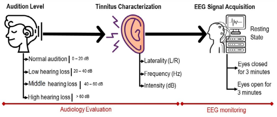
Table 1 shows the central tendencies of audiometry and tinnitus characterization. As can be seen from the table, most participants had unilateral tinnitus around 6 kHz with an approximate intensity of 16 dB. The control group presented a normal audition. With respect to EEG activity, signals were recorded to estimate the tonotopic cortical reorganization owing to neural synchrony abnormalities that provokes tinnitus.
Table 1 Shows the central tendencies of audiometry and tinnitus characterization. As can be seen from the table, most participants had unilateral tinnitus around 6 kHz with an approximate intensity of 16 dB. The control group presented a normal audition. With respect to EEG activity, signals were recorded to estimate the tonotopic cortical reorganization owing to neural synchrony abnormalities that provokes tinnitus.
| Men | Women | Tinnitus Laterality | Tinnitus Frequency | Intensity | ||
|---|---|---|---|---|---|---|
| Left | Right | Both | {kHz} | dB | ||
| 11 | 13 | 6 | 7 | 5 | 5.875 | 15.93 |
| ±2698 | ±10.68 | |||||
Analyzing the neurophysiological signals can help to diagnose and to treatment neurological diseases like tinnitus56. EEG signals were registered in calm (in two stages: eyes closed (EC) and open (EO)) for 180 seconds (each stage). To register EEG signals, a g. USBamp was employed, with 16 EEG channels, this is a high-performance and high-accuracy biosignal amplifier for the acquisition and processing of physiological signals and it was set up to record signals with 256Hz of sampling frequency and a bandwidth of 0.1 to 100 Hz. The Cz channel was the reference with respect to the international 10-20 system, and ground was the left lobe ear.
Electrode and Frequency Band Selection
The EEG analysis was focused on frontal (Fz) and occipital (O1 and O2) lobes within two bandwidths: delta (0.1-4 Hz) and alpha (7-14 Hz) band, respectively. Frontal delta activity has been extensively discussed as a major EEG abnormal synchronicity for tinnitus and neuropathic pain, and occipital alpha activity is the dominant synchronicity at resting state condition in the human beings. Note that temporal lobe was not considered for the analysis, although it is associated with auditory processing and perception of language. It is well known that temporal lobe is around 18 % of the size of the complete cortex, 17 % in the right hemisphere and 18 % in the left hemisphere. However, a large surface of the temporal lobe is into the temporal gyrus, what nullified dipoles and minimizes EEG magnitude.
EEG Signal Preprocessing
To preprocess EEG signals, EEGLAB toolbox for Matlab was used. The principal objective of signal cleaning is to maximize the dynamic range by deleting internal and external unwanted sources such as line interference, involuntary movements, cardiac and muscular signals. The procedure was divided into 5 steps: 1) baseline suppression, 2) IIR Butterworth filter from 0.1 to 100 Hz. Note that this digital filter was applied, even when a previous similar filter had been applied in the signal acquisition process. Owing to some OpenViBE bugs during the acquisition that randomly filtered the signals, the filtering process was guaranteed in the preprocessing stage, 3) IIR Butterworth filter to reject 60 Hz component, 4) transient artefacts rejection (which refer to unexpected change of signal trajectory due to electrode pop-ups or cable movements) by artifact subspace reconstruction (ASR) algorithm (this approach learns a statistical model on clean calibration data and reduce unwanted signal by dividing small segments of EEG signals and comparing them in the component subspace), 5) automatic elimination of stationary artefacts (which refer to periodic or quasiperiodic biological (such as ocular and cardiac activity) or nonbiological (line noise) signals) by the compound algorithm based on wavelet decomposition and independent component analysis (ICA).
EEG Signal Processing
Having cleaned EEG data, different processing steps were performed depending on the domain analysis (time or frequency).
For time-domain analysis, each signal:
Was filtered on Alpha (7 - 14 Hz) and Delta; (0.1 - 4 Hz) frequency bands
Was segmented into 2s time-windows without over-lap, resulting in 30 windows per signal.
For frequency-domain analysis, each signal:
Was segmented into 2s time-windows without over-lap, resulting in 30 windows per signal.
For each window, the magnitude frequency spectrum using the fast Fourier transform algorithm was computed.
Specific frequency bands from magnitude frequency spectrum were selected, this is, Alpha (7 - 14 Hz) and Delta (0.1 - 4 Hz) bands.
To this point, a dataset of 300 instances for every participant was produced; this is, 2 bands × 5-time courses (Fz, O1 and O2 channels plus bipolar O1−O2 and aver-age (O1 + O2)/2) × 30 windows. Finally, all participant instances were characterized using time and frequency domain features.
EEG Feature Extraction
Feature extraction is the process that allows obtaining information about data. It can be performed in several manners (i.e., time-domain -data samples domain- or frequency-domain -analyzing time-frequency data representations- but also in spatial-domain -spatial location of the measure-). In this work, a feature extraction in time and frequency domains for three different locations on the brain resulted in 300 instances for each participant. Thus, the feature is a combination of time-domain or frequency domain metric with a specific brain location of the brain denoted by the electrode placement. Below, different metrics in different domains are presented. Basic Statistical Measures section presents basic statistical metrics used for both time and frequency domain. Time Domain and Frequency Domain sections describe how each statistical metric could be interpreted and additional non-statistical metrics.
Basic Statistical Measure
Mean. The mean is one of the measures of central tendency that gives us information about the average value of the set of amplitude values over the number of samples of a signal (see Equation 1).
where xi correspond to the ith position of the signal, N is the sample size, and
Standard Deviation (STD). The standard deviation is a measure that tells how dispersed the values of the signal samples are with respect to their mean, being a value close to zero an indicator that the values are very close to the mean value and much higher values are an indicator that these values are further from the mean value. In other words, STD is the square root of the average of the squared differences from the Mean (see Equation 2).
where xi correspond to the ith position of the signal, N is the sample size, and x the average value58.
Kurtosis (KRT). Kurtosis is a measure that reveals the peak or flatness of a distribution. To calculate the kurtosis value, it is necessary to use Equation (3), which considers the difference of the signal data with respect to the mean59.
Skewness (SKW). Its value is zero when it has a symmetric distribution and as some non-zero value when it has an asymmetric distribution compared to the baseline60. To calculate the value of the skewness, it is necessary to use Equation (4), which considers the dispersion of the signal data with respect to the mean.
Time Domain
Time domain or data samples domain is a representation of how data is organized after acquisition step. Simple measurements on this data representation can be done to obtain some information. These basic measurements are the same that are used in statistics for data sequences. Thus, time domain features are very related to statistical features. In the next paragraphs a description of non-statistical measures is presented.
Time domain statistical measures such as mean, standard deviation, kurtosis and skewness (see Basic Statistical Measures section) describe tendencies in the time domain. For example, EEG data basic statistics, such as mean and standard deviation (see Equations 1 and 2), computed for each time window, describe how the average of EEG amplitudes change from one window to another (Mean) along with their dispersion (STD). On the other hand, there are more elaborated statistics such as kurtosis and skewness (see Equations 3 and 4). Kurtosis indicates if EEG amplitudes consist of isolated peak values (positive kurtosis) or consist of low frequency (negative kurtosis) while Skewness indicate the degree of symmetry deviation from a normal or Gaussian distribution (skew) of EEG amplitudes and if this change from one window to another. Non-statistical measures can be used as time domain descriptors. For example, the maximum amplitude of the signal (a.k.a maximum peak) and the shape which is a descriptor of the symmetry, number of peaks, obliquity, and uniformity of a measured signal. In the next lines, the equations for these features are presented.
Maximum Peak (MPK). The maximum peak corresponds to the instantaneous absolute value of the higher amplitude of the signal measured from the zero level. This metric is expressed by Equation (5).
Where xi corresponds to the ith position of the signal with i ∈ {1, 2, 3, ..., N} and N being the sample size. Finally, xpeak corresponds to the maximum peak.
Shape (SHP). Shape is not precisely a statistical parameter but is a measure that describes the characteristics of symmetry, number of peaks, obliquity, and uniformity of a signal. To calculate it, the root mean squared amplitude value must be divided by the mean absolute value (see Equation (6)).
Other data representations, such as frequency-domain, can also benefit from these statistical measures to describe the frequency spectrum. In the next paragraphs, the statistical descriptors used in frequency domain are presented.
Frequency Domain
In the frequency domain, statistical measures such as the mean and skewness can be used as descriptors. For example, in the case of EEG signals, the Mean of a signal segment obtained for each one of several magnitude spectrum windows can tell us how the average of EEG spectrum (energy) changes from one window to another. On the other hand, more elaborated statistics such as the skewness can explain the degree of deviation from symmetry from a normal or Gaussian distribution (skew) of the EEG spectrum and, if exist a change from one window to another. Other measures can be used as frequency domain features and are described as follows.
Power Spectral Density (PSD). The PSD refers to distribution of spectral energy observed in each unit time. This total power can be calculated by performing the summation or integration of the spectral components which, as dictated by Parseval’s theorem60.
where s(k) is a spectrum for k = 1, 2, ..., K, K is the spectrum resolution61)(62)(63.
P5 (MNF or Xfc). Another specific frequency spectrum metric, P5 may show how the position is changing of principal frequencies that are predominant in the frequency spectrum and is basically the sum of the product of the frequency value by its magnitude divided by the sum of the magnitudes of all the elements of the spectrum (see Equation (8)).
where s(k) is a spectrum for k = 1, 2, ..., K, K is the number of elements in the spectrum and fk is a value of the k spectrum line61)(62)(63. To perform the feature extraction, for each instance of every participant, the etrics corresponding to time and frequency domain were computed. Thereafter, the participant data were organized in a matrix shape where the rows correspond to the participant instances and the columns to different audition levels. The instances corresponding to all participants with the same audition level are concatenated one after the other. The matrices were labeled according to their information. For example, the label O2_alpha_STD corresponds to a matrix with all participant instances corresponding to the occipital 2 channel (O2), on Alpha band, characterized by the standard deviation feature (SD). Table 2 depicts an example of the matrix O2_alpha_STD.
Table 2 Example of the matrixO2_alpha_STD
| Participant | Control/Normal | Tinnitus/Low | Tinnitus/Middle | Tinnitus/ High |
|---|---|---|---|---|
| 1 | 6.299 | 4.615 | 8.474 | 4.641 |
| 1 | 6.068 | 7.491 | 6.775 | 9.594 |
| : | : | : | : | : |
| 1 | 4.334 | 8.194 | 4.507 | 5.113 |
| : | : | : | : | : |
| 6 | 6.626 | 3.757 | 4.067 | 8.462 |
| 6 | 10.058 | 6.298 | 8.395 | 10.705 |
| : | : | : | : | : |
| 6 | 5.262 | 4.18 | 3.571 | 10.977 |
To identify one or several neuromarkers that differentiate between participants with different audition levels based on their EEG signals, first, the dataset distribution and the appropriate non-parametric statistical test are determined.
Statistical Analysis
In statistical analysis it is important to know which distribution a sample is drawn from, to make correct inferences. According to the data of this study, the analysis is performed using the Lilliefors test based on the Kolmogorov-Smirnov test in R with the nortest package. The Lilliefors test for normality is an adaptation of the Kolmogorov-Smirnov test for the case when the parameters of the mean and variance of the normal distribution is unknown64. The Lilliefors test is defined by:
where Fn(x) is the empirical cumulative distribution function and F*(x) is the function of cumulative distribution of the normal distribution with μ =
All time and frequency metrics were analyzed using the Kolmogorov-Smirnov test with the Lilliefors correction, showing p<0.05. Consequently, the normality hypothesis is rejected. The nonparametric technique to test whether the populations differ in location, the Kruskal-Wallis H statistic analysis does not require actualized observation values, the ranks of the observations to complete the analysis is known. The test of Kruskal-Wallis is based on H for comparing k population distributions65:
H0: The distribution of k population is the same.
Ha: The population distributions differ in two locations.
Test statistic:
Results and discussion
After statistical analysis, the bipolar O1 − O2 and the average (O1 + O2)/2 produced nonsignificant differences in alpha nor in delta; thus, they were not further analyzed. Only the results from 180 out of 300 sets (2 bands × 3 channels (Fz, O1 and O2) × 30 windows) are reported here. To evaluate the performance of every feature and its possibility to become a neuromarker, two different strategies were pursued. First, a depiction of the probability distribution of the data using violin plotting along with a statistical summary using box plots are presented (Figures 4 to 3). Secondly, an statistical significance analysis was performed with the Kruskal-Wallis test and reported on Tables 3 and 4. The data distribution for features Fz-delta-MPK and Fz-delta-STD respectively in the time domain for delta band and electrode Fz among the studied groups are observed in Figures 2 and 3. Apart from the skewed distribution of these two features it can be easily observed that Fz-delta-MPK and Fz-delta STD distributions in each group looks very similar as it was for electrode O2 in the alpha band for the same features. Looking into distributions of Fz-delta-MPK and Fz-delta-STD features, we can easily observe that median value.
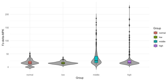
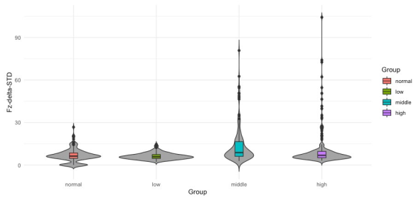
Table 3 P-values for Time-domain analysis on Delta band and Fz channel
| Feature | Audition Levels | ||||||
|---|---|---|---|---|---|---|---|
| Channel | Metric | Tinnitus/Low vs Control/Normal | Tinnitus/Middle vs Control/Normal | Tinnitus/Middle vs Tinnitus/Low | Tinnitus/High vs Control/Normal | Tinnitus/High vs Tinnitus/Low | Tinnitus/High vs Tinnitus/Middle |
| Fz | MPK | - | 3.5 x 10⁻¹³ | 2 x 10-16 | 0.0041 | 2 x 10-16 | 0.0001 |
| Fz | STD | - | 1.3 x 10⁻⁹ | 1.1 x 10⁻¹⁴ | - | 0.0004 | 0.0005 |
Table 4 P-values for Frequency-domain analysis on alpha band
| Feature | Audition Levels | ||||||
|---|---|---|---|---|---|---|---|
| Channel | Metric | Tinnitus/Low vs Control/Normal | Tinnitus/Middle vs Control/Normal | Tinnitus/Middle vs Tinnitus/Low | Tinnitus/High vs Control/Normal | Tinnitus/High vs Tinnitus/Low | Tinnitus/High vs Tinnitus/Middle |
| O2 | PSD | 0.0251 | 2.1 x 10⁻¹¹ | 7.7 x 10⁻⁶ | 6.4 x 10⁻⁷ | 0.0002 | - |
| O2 | STD | 0.036 | 8.9 x 10⁻¹⁴ | 4.2 x 10⁻¹⁰ | 3.7 x 10⁻¹⁰ | 5.2 x 10⁻⁷ | - |
| O2 | MPK | 0.039 | 2.3 x 10⁻¹³ | 3.9 x 10⁻⁹ | 5.0 x 10⁻⁹ | 4.4 x 10⁻⁶ | - |
| O1 | SHP | 2.2 x 10⁻¹⁶ | < x 10-16 | 9.1 x 10⁻⁵ | 8.9 x 10⁻⁵ | 8.0 x 10⁻⁵ | |
| O1 | SKW | 1.9 x 10⁻¹⁰ | 2.9 x 10⁻¹¹ | 3.1 x 10⁻³ | 0.0037 | 0.0033 | |
from normal group differs significantly from the median value of group middle. It is hard to see but there are also significant differences between median values of groups low and middle and middle and high for both features. However, in the case of Fz-delta-STD there are not significant differences between the median values of groups normal and high as there are present for the case of Fz-delta-MPK (see Table 3, fifth column). In Figure 4 to 6, the data distribution for features O2-alpha-PSD, O2- alpha-STD and O2-alpha-MPK in the frequency domain for alpha band and electrode O2 among the studied groups is shown. Apart from the skewed distribution of these three features and the longer tails for O2-alpha-PSD feature, it can be easily observed that O2-alpha-STD and O2-alpha-MPK distributions in each group looks very similar. Nevertheless, if it can be looked carefully out of its tails, distribution for O2-alpha-PSD is almost proportional to O2- alpha-STD and O2-alpha-MPK distributions with exception of normal group.
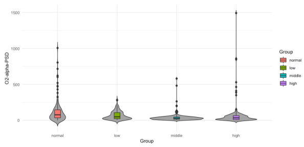

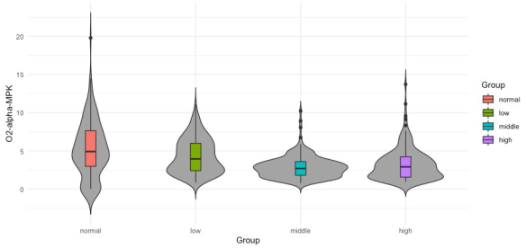
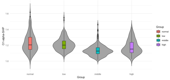
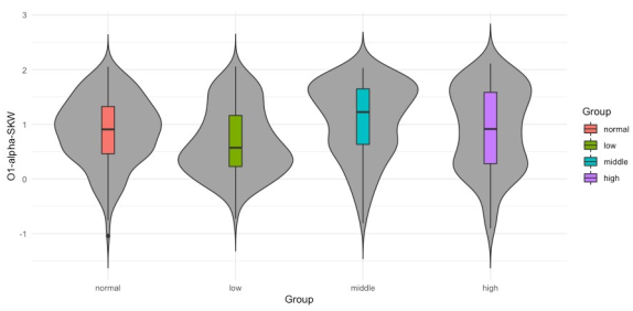
However, for the three groups it seems that median value from normal group differs significantly from the median values of groups middle and high. Also, is possible to observe that median values of middle and high groups differ significantly from the median of group low. It is hard to visually determine if the medians of groups normal and low possess significant differences. However, there exist significant differences as confirmed in the third column (Tinnitus/Low vs. Control/ Normal) of Table 4 where p-values of 0.0251, 0.036 and 0.039 report significant differences for groups normal and low. It can be also observed that medians from groups middle and high are not significantly different, which is also confirmed in Table 4 in the last column (Tinnitus/High vs. Tinnitus/Middle) where there are no p-values reported since only p-values lower than 0.05 are presented. In Figures 7 and 8 the data distribution for features O1-alpha-SHP and O1- alpha-SKW respectively in the frequency domain for alpha band and electrode O1 among the studied groups is presented. Apart from the skewed distribution of these two features it can be easily observed that O1-alpha-SHP and O1-alpha-SKW distributions in each group look very different. Nevertheless, if it can be looked carefully for both O1-alpha-SHP and O1-alpha-SKW features, the median value from normal and low groups differs significantly from the median value of groups middle and high. Visually from these plots, it is easy to see that median values of groups normal and low do not possess significant differences (Table 4 third column, no p-values are reported); however, it can be easily observed that median values from groups middle and high are significantly different. In the other hand, significant differences between median values of normal and high groups are only difficult to be observed from plots for O1-alpha-SKW feature, but there exists as reported in Table 4 sixth column, p-value equal to 3.1 × 10⁻³.
Tables 3 and 4 present time and frequency features (combination of the frequency band, channel, and metric) that first, maximizes the differences between groups of participants with different audition levels and second, fulfills the criteria of p < 0.05, for time and frequency domain, respectively. Based on the concept that the ideal neuromarker would be a metric in a data domain for a specific location capable to distinguish among all groups, each group was compared to another (i.e., all non-repeated pairs of groups), testing the features obtained for time and frequency domains for specific head locations to grade the easiness for such a feature to distinguish among groups.
Many features are helpful to distinguish among several groups; however, the interest is only in features capable of distinguishing most of the groups. In our study, apparently it is observed that for time-domain and frequency-domain there is no such a metric capable of distinguishing the six groups presented here. Nevertheless, some metrics were found in the frequency domain that in combination with a channel location are capable to distinguish 5 out 6 groups and in the time domain only with the MPK metric is possible to distinguish 5 out 6 groups with a p value < 0.05. Tables 3 and 4 present only the features that meet this number of groups distinguished with this significance. From Table 3 it is observed possible neuromarkers in the time domain, all of them are located on the frontal lobe and described by two metrics on the delta band. These metrics are the standard deviation (STD) and maximum peak (MPK), being the latter the one that can help us to distinguish at least 5 out of 6 groups presented here. In addition, on Table 4 it is observed features identified as possible neuromarkers in the frequency domain, all of them are located on the occipital lobe and described by several metrics on the alpha band such as its power spectral density (PSD), standard deviation (STD), maximum peak (MPK), shape (SHP) and skewness (SKW). As seen in Table 4, the shape (SHP) and skewness (SKW) of the alpha frequency band does not present significant differences between Tinnitus/Low and Control/Normal groups of subjects; on the other hand, PSD, STD, and MPK did not present significant differences between Tinnitus/High and Tinnitus/Middle groups. However, if we consider the occipital lobe as one region for which we have two measurements, we can distinguish among the six groups presented here using a different metric for each side of the occipital lobe.
The non-significant differences among Tinnitus/Low and Control/Normal groups of subjects for SKW metric in the alpha band could be since SKW explains the degree of deviation from symmetry from a normal or Gaussian distribution (skew) of the EEG spectrum. In this case, as it was presented before (see Frequency Domain section) the data distribution of the tested metrics in all groups was non Gaussian which implies the existence of similarities between groups from the point of view of this metric. Metrics such as PSD, STD and MPK in the frequency domain gives information about power differences in a frequency band (i.e., there are certain frequencies that prevailed). Thus, it is possible that the group Tinnitus/High and Tinnitus/Middle share some frequencies maybe related to tinnitus, and in this context from the point of view of this metric is impossible to distinguish between both groups. Regarding these results, frequency domain metrics seem to be more robust than time domain metrics because they can help to distinguish more different groups than most of the time domain metrics tested here. However, it is important to remark that both frequency and time domain metrics can be used together to distinguish among groups. For example, by analyzing MPK metric in both domains over their respective EEG channels Fz and O2 at the same time, it is possible to distinguish both Tinnitus/Low vs Control/Normal and Tinnitus/High vs Tinnitus/Middle, which is not possible if we analyze the feature in one domain only. The non-Gaussian distribution of data for the metrics presented here makes that parametric statistical test such ANOVA cannot be used in this analysis and thus, equivalent non-parametric tests need to be used.
Other options are transforming data with a function forcing it to fit a normal model and then applying ANOVA or another parametric test. However, when data distribution is skewed and fitting another distribution type as in our case, it is recommendable to use non-parametric tests (i.e., these tests do not assume that data fits a specific type of distribution). Even though it has been presented several neuromarkers distinguishing control participants with no HL from tinnitus participants with some level of HL, and tinnitus participants with different levels of HL among them. These neuromarkers identify significant differences between instances by analyzing one feature.
Additionally, the effectiveness of using a particular neuromarker for tinnitus or HL level estimation cannot be assessed. Therefore, based on results of the present work, and as a future work, these features will be used along with several machine learning techniques to first, evaluate the performance of the combination of the neuromarkers proposed here for predicting tinnitus condition or HL level on participants; finally, the evaluation of the efficiency of such predictions will be performed.
Conclusion
A methodology to characterize and identify subjects from different audition levels (Normal, Low, Middle, and High) was presented. The results show that it is possible to perform a pairwise differentiation of patients with different HL conditions in both time and frequency-domain. It was shown that the resulting EEG characterization does not fit the normal probability distribution, so the Kruskal-Wallis test was required to measure the significant difference between pairwise combinations. There are more metrics in the frequency-domain that allow differentiating audition levels than those from the time-domain; with MPK and STD being shared by both domains. The results indicate that for every audition level pairwise comparison, there is at least one combination of an electrode, band, and metric (feature) in which such pairwise combination is differentiable. On frequency-domain on the Alpha band, PSD, STD, and MPK are neuromarkers that distinguish a Control/Normal subject from a Tinnitus participant with Low, Middle, and High audition level. And, to distinguish from different tinnitus audition level participants, SHP and SKW are the neuromarkers to be selected. Moreover, combination of both domains allows to distinguish among all the groups presented here as is the case of metric MPK (Fz-Delta-MPK, in time domain and O2-Alpha-MPK in frequency domain).
It's important to note that tinnitus is a subjective experience, and its perception can vary greatly among individuals, regardless of age. Some individuals may habituate to the sound and experience minimal distress, while others may find it highly bothersome and experience significant negative effects on their well-being. Additionally, individual characteristics, such as personality traits and psychological factors, can influence how tinnitus is perceived and coped with, irrespective of age.
A small sample size may limit the generalizability of the findings and reduce the statistical power of the analysis. Or maybe using machine learning techniques to distinguish between different groups. To draw more reliable conclusions, a larger and more diverse sample should be used in future studies. The outcomes of this study are specific to the parameters and methods used in this research. The same neuromarkers and metrics to different populations or other hearing disorders cannot be generalized. Replication of the study with different populations and in different settings would help assess the generalizability of the results.

