


 nueva página del texto (beta)
 Inglés (pdf)
 Artículo en XML
 Referencias del artículo
 Enviar artículo por email
 Citado por SciELO
  Similares en
SciELO
Similares en
SciELO 
 Permalink
Introduction
One of the most interesting applications for Brain-Computer Interfaces (BCIs) is the P300 speller, proposed in 1988 by Farwell and Donchin [1] and re-invented and improved in many other studies [2] [3] [4] [5]. A commonly used speller consists of an arrangement of characters uniformly distributed in rows and columns, displayed in a screen. Rather than displaying a single character, the speller randomly highlights some characters organized in rows or columns. When the user watches the desired character in a highlighted row or column, the brain generates a P300 signal, related to memory and the attention processes in the brain [6].
A typical P300 speller reads signals from the brain, using electroencephalography (EEG), and tries to discriminate between P300 and non-P300 signals. When a P300 signal is detected in a specific row and column, the speller takes the corresponding character and displays it on the screen. The described speller has been used for developing online BCI applications [5] [7] [8] [9]. Note that the target of the classification is to identify the row and the column that corresponds to a character from P300 signals rather than to classify P300 and non-P300 signals.
As the P300 speller is based in the oddball paradigm, the number of events is unbalanced; that is, the number of non-P300 trials is larger than the number of P300 trials [10]. Both unbalanced classes and small datasets could affect the performance measurement of a classifier [11] [12]. To get a more confident performance, the number of samples by class should be balanced.
Some researchers have proposed discarding samples randomly from the class with more members to reach the desired 1:1 proportion [13] [14] [15] [16] [17], trying to preserve as many samples as possible in the training stage [18]. This solves the problem of unbalanced classes at the expense of decreasing the number of available samples.
By contrast, there are mainly three approaches to processing the input features to a classifier for a P300 speller. The first one consists of training and evaluating the classifier in single trials [3] [8] [19]. The second approach makes use of averaged data over a fixed number of trials, for training and testing the system [5] [7] [9] [13] [16] [20] [21] [22]. The third approach consists of training the classifier in single trials, and evaluating the classifier with averaged trials [14] [17] [23] [24].
The last approach (called the traditional approach in this work) is commonly used in the literature. It suffers from an important problem of statistical properties of signals during the training stage being different from those of signals used during the testing stage. This violates the assumption that training and testing data should come from the same population, for any classification problem [25]. Consequently, the classifier has reduced capacity to differentiate between P300 and non-P300 trials.
Different statistical properties of training and testing signals carry another problem. The estimation of the posterior probabilities from probabilistic classification approaches would not be correct.
This issue is critical for P300 applications that make use of language models [7] [26] [27] [28] since the posterior probability of the output of the classifier is typically combined with the probability of letters in a particular language to determine the most likely sequence of letters.
In addition, since P300 and non-P300 classes are unbalanced, performance measures, such as the accuracy, tend to be biased. This happens because the classifier assigns most of the samples to the class with higher prior probability [12]. Some studies have proposed use of the Cohen's kappa index κ as an alternative measure of performance that does not suffer from the issues previously described [29] [30] [31].
The classification problem could be seen from one of two possible points of view. The first one establishes that the classification problem is typically divided into two stages. The inference stage tries to learn a probabilistic model of the data given the class. Then, the decision stage implements the theorem of Bayes to determine the class of each data. A classifier implemented in this manner is known as a generative classifier [25]. Linear discriminant analysis (LDA) classifiers are generative because they mostly assume Gaussian distributions in the data [25] [32].
The second point of view determines that a class could be directly mapped from the data. The model comes from either a probabilistic discriminant model of the class, given the data, or a deterministic discriminant function that directly maps the data to the class. A classifier that uses the latter approach is a discriminative classifier [25]. Logistic regression and the support-vector machine (SVM) are examples of discriminative classifiers that use a probabilistic model and a discriminant function, respectively.
In this work, a method for training linear classifiers in the identification of P300 potentials is presented. First, we demonstrate that the traditional approach could lead to misinterpretation of the actual performance of these classifiers, as the performance metric based on accuracy is not well suited for the cases of unbalanced classes. Second, a bootstrapping approach is presented as a method for obtaining effective training of linear classifiers. Results indicate a significant improvement using the proposed method for detection of P300 potentials.
Methods
Experiment and dataset description
The experiment consists of declaring one of 36 possible characters (26 letters and 10 digits). Each subject observed a 6 × 6 matrix of characters in a screen, focusing the attention on the character that was prescribed above the matrix speller. For each character, the matrix was displayed for a 2.5 s period, and all characters had the same intensity. Afterward, each column and each row were randomly intensified for 100 ms, followed by a blank period of 75 ms after each intensification step. There were 12 different row/column stimuli by round and 15 rounds of intensifications by character, for a total of 31.5 s. Each subject spelled 32 characters in total. Fourteen healthy subjects participated in the study.
The dataset contains EEG signals that were recorded using a cap embedded with 64 electrodes, according to the modified 10-20 system [33]. All electrodes were referenced to the right earlobe and grounded to the right mastoid. The raw EEG signal was bandpass-filtered between 0.1 and 60 Hz and amplified with a 20000X SA Electronics amplifier [23]. Each experiment took into account only 16 EEG channels, motivated by the study presented by Krusienski et al. [23]: F3, Fz, F4, FCz, C3, Cz, C4, CPz, P3, Pz, P4, PO7, PO8, O1, O2, and Oz. Each channel is sampled at a rate of 240 Hz for one subject and 256 Hz for the others. All aspects of the data collection and experimental control were controlled by the BCI2000 system [22]. Two datasets were acquired for each subject: One was used for training, and the other was implemented for testing. Both databases were taken on different days. All datasets were obtained from the Wadsworth Center, NYS Department of Health.
Data processing
Data were pre-processed using bandpass filtering, separation in trials and decimation. Then, all channels were concatenated in a single vector. Depending on the type of training, data were taken from either the input of a classifier or a new population for obtaining new samples. In the latter case, a determined number of N averaged samples were taken. Afterward, the training datasets were inputs of a linear discriminant classifier. Details are explained in the following subsections.
Pre-processing
For each subject, data were bandpass-filtered between 1 and 20 Hz using a fourth-order Butterworth filter. The chosen bandwidth eliminates the trend of each channel and allows decimation of the signal later, by preventing the aliasing. Afterward, data were separated in trials by taking a window of 600 ms after the presentation of each visual stimulus (the highlight of one row or column), as proposed in a previous work [26]. Signals from all channels were decimated by a factor of 4 and concatenated in a single feature vector. The factor was chosen because frequencies higher than that of the beta band reflect unrelated neural processes to P300 in awareness [34]. In addition, the maximum analog frequency of the EEG signal is 60 Hz, as seen before [23]. For the averaged process, signal segments were averaged across repetitions, up to the maximum number of repetitions by character (15). Concatenated channels were used as the inputs of the classifier since they are used in the traditional method, as described in [23].
Re-sampling of training samples
In the traditional approach, the classifier is trained with single trials and tested on averaged trials, to increase the signal-to-noise ratio. Note that besides the issue of having unbalanced data, the statistical properties of the training data do not match those of the testing data.
To avoid these problems, we implement an approach based on bootstrap re-sampling (bootstrapping) [32] [35]. From the training trials, a new dataset is obtained by re-sampling N trials with replacement, where N is the number of trials used to get an averaged sample. The process is repeated M times by class, to get M averaged samples by class. The new dataset is used to train a classifier such that 1) the number of samples is equal for each class in the training set, and 2) the statistical properties of training and testing data remain comparable. It is worth noting that in practical scenarios, the number of averaged trials may not be defined a priori. However, this procedure can be followed for any value of N. Additionally, it does not imply any additional significant computational load, as the re-sampling is computationally inexpensive.
In this work, we used the training dataset as a new population to implement the re-sampling. We varied the number of repetitions (single trials) used to get a new averaged trial, with N = {2, 3, ..., 14, 15}, because 15 is the maximum number of repetitions available by character. Then, we repeated the process M times by class. Single trials were not used because re-sampling only allows obtaining repeated samples, decreasing the variability of the training samples in the mentioned case.
We tested a classifier trained with one of the following kinds of samples: unbalanced classes with single trials and balanced classes by re-sampling M = {1000, 2000, 3000} averaged trials by class. The value of M is chosen according to the statistical significance obtained in the results, for all the classifying algorithms. For all cases, averaged trials were used as testing data.
Classifiers
In the literature, the classification problem involves identifying the row and the column that corresponds to a character of the speller. In the present study, the target of the classification is to determine whether a signal is P300 or not. For aiming to the goal, we implemented four classifying algorithms in the study: step-wise linear discriminant analysis (SWLDA), Bayesian linear discriminant analysis (BLDA), support-vector machine with a linear kernel (LSVM) and logistic regression (Log Reg). While LDA-based algorithms are generative classifiers, LSVM and Log Reg lies in the category of linear discriminative classifiers [25] [36]. The results presented are based on the test datasets, which are not seen by any of the implemented classifiers during the training procedure.
For discriminative classifiers, it is necessary to choose the value of a regularization factor C. A four-fold cross-validation process is implemented with the training dataset, to get the best value of C. The number of values tested for C was 25, all located between 0.01 and 1. After this procedure, the final classifier is trained using the whole training dataset and the chosen value of C. The process is repeated by each user and each type of training samples [36].
Stepwise LDA
The traditional approach implements a modified version of LDA as the classifier, where a stepwise regression is used before the classification task [23]. The classifier is known as SWLDA. Unlike other LDA-based classifiers, this classifier chooses the coefficients of the model regression iteratively, according to a statistical criterion [37]. As a result, the model obtained is more compact than the least-squares-based regression. The study implements the stepwise regression included in the Statistical and Machine Learning Toolbox for MATLAB®. Additional details of SWLDA can be found in [38].
Bayesian LDA
When the coefficients of the model implemented for LDA are chosen according to Bayesian criteria, an LDA classifier based on Bayesian interpolation (BLDA) is obtained. According to the literature, the algorithm gives better results than the ordinary LDA or, even, SWLDA [39] [40]. Like the SWLDA classifier, the coefficients are obtained by iteration. However, the statistical criteria for choosing corrections are based on the Bayes Rule and are not added or removed from the model [41]. The algorithm implemented in the study and further details of BLDA can be obtained from [39].
Linear SVM
Support-vector machine (SVM)-based classifiers have been implemented in several previous studies related to BCIs, including P300 spellers [14] [15] [20] [42] [43]. In this work, a linear kernel support-vector machine was implemented as the classifier with the LIBSVM Toolbox for MATLAB® [44], for each subject. The reader is encouraged to see [45] for a wide list of studies implementing SVM in BCIs.
Logistic Regression
Unlike the L-SVM, logistic regression-based classifiers have been implemented in fewer works related to BCIs [46] [47]. It is a member of the family of log-linear models, implemented in discriminative classifiers [25] [32]. In the present study, the classifier was implemented with the UGM Toolbox for MATLAB® [48], for each subject. Further details about Logistic Regression are found in [25].
Accuracy
A common measure of performance used for classification is the accuracy. Accuracy is defined as a metric of the closeness between measured or predicted values and their corresponding true values [49]. A measure commonly used for the accuracy, for classification problems with M_c classes, is defined by using the trace of a confusion matrix H [29] as shown indicated in Equation ( 1 ):
Where where Ns is the total number of samples entered to the classifier, and trace(H) is the number of samples correctly classified. Accuracy varies from 0 to 1, where 1 gives represents a perfect classification.
Since the definition of accuracy is closely related to the definition of the
binomial distribution
However, high accuracy does not always mean the classifier has high performance. This is true when the number of classes is highly unbalanced, as the classifier tends to be biased toward the class with the highest occurrence in the dataset. This is known as the accuracy paradox [50].
Cohen’s kappa index
A commonly used measure of precision is the Cohen's kappa index κ [29] [51] [52]. It is an alternative way of measuring the predictive power of a classifier that relates the accuracy with the probability to classify by chance, as expressed by Equation (3):
The numerator is the difference between the accuracy and the expected probability to classify correctly by chance (pe). The denominator is the difference between the maximum accuracy and pe . Consequently, κ is defined as the rate of the difference between accuracy and pe , and the maximum value of this difference is used to determine the difference. The possible values for κ are within the range of −1 to 1 [53]. A value of 1 means perfect classification, whereas a value of 0 indicates random assignments between true classes and the predicted values. Finally, a value of −1 indicates an opposite relationship between the real and predicted values. The expected probability pe is defined in the Equation (4):
Where the sum of all elements for an the i-th row ni: and the sum of all elements for an the i-th column n:i are expressed in Equations (5) and (6) [30]:
The standard deviation of κ is calculated using Equation (7):
The standard error can be used to build confidence intervals and calculate statistical significance when accuracy or kappa values are compared.
Results
Results presented here refer to the average performance obtained by each classifier, in terms of the accuracy and Cohen's kappa index metrics. All metrics were obtained from the testing dataset of each subject.
Number of bootstrapped samples
The statistical significance of differences among the numbers of bootstrapped samples for averaged training data was tested by a one-way randomized blocks ANOVA using a performance index and a classifier. ANOVA was chosen rather than a Student's t-test because ANOVA does not take into account the random effects of the number of averages and subjects, whereas ANOVA does. The number of training data (M) was taken as the design variable, and each performance index was the output variable. Subjects and the number of averaged samples by a testing trial were taken as randomized blocks. The numbers of samples used were M = {1,000, 2,000, 3,000}.
For Log Reg, the ANOVA test does not give any significant differences among the number of bootstrapped samples for neither accuracy nor Cohen’s kappa index (accuracy: F = 1.72, p = 0.18; Cohen's kappa index: F = 0.51, p = 0.60). In the case of LSVM, there is no statistical difference in the number of samples (accuracy: F = 0.92, p = 0.40; Cohen's kappa index: F = 0.02, p = 0.98). Similar conclusions are obtained by analyzing the results of ANOVA tests for SWLDA (accuracy: F = 0.61, p = 0.55; Cohen's kappa index: F = 0.13, p = 0.88) and BLDA (accuracy: F = 0.67, p = 0.51; Cohen's kappa index: F = 0.39, p = 0.25). Although there is no significant difference, most of highest results were obtained with M = 2,000 averaged bootstrapped samples. Therefore, the chosen number of samples is M = 2,000 in the remaining sections of the paper.
Type of training samples
The statistical significance of differences among the previously described types of training data was tested by two procedures. First, a one-way randomized blocks ANOVA was performed by metric and classifier. The type of training data (traditional or proposed) was taken as the design variable. Other parameters are the same as those in the previous subsection. Then, a Student’s t-test was performed individually for each subject, by pooling the metrics and their corresponding standard deviations. The purpose was to estimate the significance of the differences between the traditional method and the proposed one, both at a general level and by each subject.
Linear SVM
Figure 1 illustrates the average performance obtained by employing the LSVM classifier on each subject and type of training data. The ANOVA test gives significant differences for both metrics (accuracy: F = 216.92, p < 0.01; Cohen's kappa index: F = 1380.10, p < 0.01). According to the results, when the classifier is trained with 2,000 averaged trials by class, the performance is significantly better than that of the traditional approach.
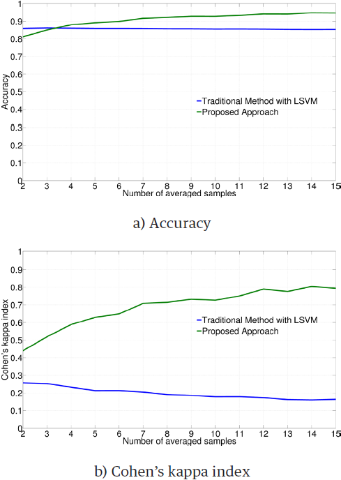
Table 1 contrasts the average of results and pooled standard deviations obtained by subject, for accuracy and kappa. A Student’s t-test was performed to get the statistical significance of the difference between the methods. Results indicate that the difference is highly significant (p < 0.01), for most of metrics and subjects. In most cases, the difference is in favor of the proposed method.
Table 1 Averaged metrics by subject, for LSVM.
| Subject | Traditional Approach | Proposed Method | ||
| Accuracy | Kappa | Accuracy | Kappa | |
| 1 | 0,95 ± 0.11 | 0.78 ± 0.33 | 0.98 ± 0.08* | 0.93 ± 0.33* |
| 2 | 0.88 ± 0.12 | 0.43 ± 0.27 | 0.95 ± 0.10* | 0.83 ± 0.33* |
| 3 | 0.84 ± 0.13 | 0.01 ± 0.07 | 0.90 ± 0.12* | 0.55 ± 0.33* |
| 4 | 0.84 ± 0.13 | 0.06 ± 0.18 | 0.95 ± 0.10* | 0.81 ± 0.30* |
| 5 | 0.88 ± 0.12 | 0.36 ± 0.26 | 0.97 ± 0.08* | 0.90 ± 0.30* |
| 6 | 0.83 ± 0.13 | 0.00 ± 0.00 | 0.84 ± 0.13 | 0.52 ± 0.27* |
| 7 | 0.83 ± 0.13 | 0.00 ± 0.00 | 0.87 ± 0.12* | 0.48 ± 0.27* |
| 8 | 0.83 ± 0.13 | 0.00 ± 0.00 | 0.87 ± 0.12* | 0.59 ± 0.28* |
| 9 | 0.89 ± 0.12 | 0.43 ± 0.27 | 0.94 ± 0.10* | 0.81 ± 0.29* |
| 10 | 0.84 ± 0.12 | 0.06 ± 0.15 | 0.94 ± 0.10* | 0.79 ± 0.30* |
| 11 | 0.85 ± 0.13 | 0.18 ± 0.22 | 0.94 ± 0.10* | 0.80 ± 0.29* |
| 12 | 0.83 ± 0.13 | 0.00 ± 0.00 | 0.90 ± 0.12* | 0.53 ± 0.28* |
| 13 | 0.88 ± 0.12 | 0.44 ± 0.27 | 0.81 ± 0.13 | 0.50 ± 0.26* |
| 14 | 0.83 ± 0.13 | 0.02 ± 0.27 | 0.90 ± 0.11* | 0.59 ± 0.29* |
| Average | 0.86 ± 0.12 | 0.20 ± 0.19 | 0.91 ± 0.11 | 0.69 ± 0.29 |
* The difference is highly significant, with a Student’s t-test (p < 0.01).
Number of samples: 372 for subject 1, 504 for the rest.
Logistic Regression
Figure 2 illustrates the average performance obtained by employing the Logistic Regression classifier on each subject and type of training data. The ANOVA test gives significant differences for both metrics (accuracy: F = 215.10, p < 0.01; Cohen's kappa index: F = 843.29, p < 0.01). Results indicate that the performance of the classifier is higher with the proposed method for training.
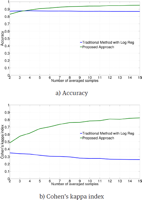
Table 2 compares the pooled results and standard deviations obtained by subject, for accuracy and kappa. Results of the Student’s t-test, by subject and metric, indicate that the difference is highly significant (p < 0.01) for most of metrics and subjects, in favor of the proposed method. The consistency in the statistical analyses for Log Reg supports the improvement in the results with our method. It also applies to the LSVM results.
Table 2 Averaged metrics by subject, for Log Reg.
| Subject | Traditional Approach | Proposed Method | ||
| Accuracy | Kappa | Accuracy | Kappa | |
| 1 | 0.97 ± 0.09 | 0.88 ± 0.33 | 0.98 ± 0.09 | 0.92 ± 0.33 |
| 2 | 0.92 ± 0.11 | 0.65 ± 0.29 | 0.96 ± 0.09* | 0.86 ± 0.30* |
| 3 | 0.84 ± 0.13 | 0.03 ± 0.14 | 0.93 ± 0.11* | 0.68 ± 0.29* |
| 4 | 0.85 ± 0.13 | 0.15 ± 0.22 | 0.95 ± 0.10* | 0.84 ± 0.30* |
| 5 | 0.91 ± 0.11 | 0.56 ± 0.29 | 0.97 ± 0.08* | 0.91 ± 0.30* |
| 6 | 0.84 ± 0.13 | 0.05 ± 0.13 | 0.86 ± 0.12* | 0.59 ± 0.27* |
| 7 | 0.83 ± 0.13 | 0.00 ± 0.07 | 0.88 ± 0.12* | 0.51 ± 0.28* |
| 8 | 0.83 ± 0.13 | 0.00 ± 0.07 | 0.88 ± 0.12* | 0.62 ± 0.28* |
| 9 | 0.92 ± 0.11 | 0.64 ± 0.29 | 0.95 ± 0.09* | 0.84 ± 0.29* |
| 10 | 0.85 ± 0.13 | 0.15 ± 0.21 | 0.95 ± 0.09* | 0.83 ± 0.30* |
| 11 | 0.88 ± 0.12 | 0.41 ± 0.27 | 0.95 ± 0.09* | 0.82 ± 0.30* |
| 12 | 0.83 ± 0.13 | 0.00 ± 0.04 | 0.90 ± 0.11* | 0.55 ± 0.29* |
| 13 | 0.91 ± 0.11 | 0.60 ± 0.29 | 0.84 ± 0.13 | 0.57 ± 0.26 |
| 14 | 0.84 ± 0.13 | 0.03 ± 0.13 | 0.91 ± 0.11* | 0.61 ± 0.29* |
| Average | 0.87 ± 0.12 | 0.30 ± 0.22 | 0.92 ± 0.11 | 0.72 ± 0.29 |
* The difference is highly significant, with a Student’s t-test (p < 0.01).
Number of samples: 372 for subject 1, 504 for the rest.
Stepwise and Bayesian LDA
Figure 3 illustrates the average performance obtained by employing the SWLDA classifier on each subject and type of training data.
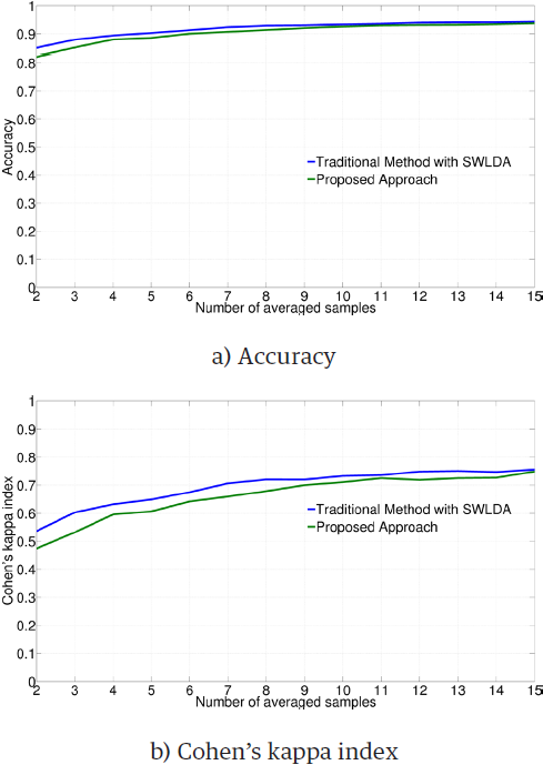
The ANOVA test gives significant differences for both metrics (accuracy: F = 28.15, p < 0.01; Cohen's kappa index: F = 20.86, p < 0.01).However, when metrics are contrasted with a Student’s t-test, results reveal that there is no statistical significance in most of the cases, as presented in Table 3.
Table 3 Averaged metrics by subject, for SWLDA.
| Subject | Traditional Approach | Proposed Method | ||
| Accuracy | Kappa | Accuracy | Kappa | |
| 1 | 0.98 ± 0.08 | 0.95 ± 0.33 | 0.98 ± 0.08 | 0.94 ± 0.33 |
| 2 | 0.96 ± 0.09 | 0.88 ± 0.30 | 0.95 ± 0.10 | 0.84 ± 0.29 |
| 3 | 0.86 ± 0.12 | 0.26 ± 0.25 | 0.87 ± 0.12 | 0.36 ± 0.26* |
| 4 | 0.95 ± 0.10 | 0.83 ± 0.30 | 0.94 ± 0.10 | 0.79 ± 0.30 |
| 5 | 0.98 ± 0.07 | 0.94 ± 0.31 | 0.98 ± 0.08 | 0.92 ± 0.30 |
| 6 | 0.88 ± 0.12 | 0.63 ± 0.28 | 0.84 ± 0.13 | 0.53 ± 0.27 |
| 7 | 0.89 ± 0.12 | 0.54 ± 0.28 | 0.86 ± 0.12 | 0.48 ± 0.27 |
| 8 | 0.90 ± 0.11 | 0.68 ± 0.28 | 0.87 ± 0.12 | 0.60 ± 0.28 |
| 9 | 0.94 ± 0.10 | 0.82 ± 0.29 | 0.93 ± 0.10 | 0.80 ± 0.29 |
| 10 | 0.94 ± 0.10 | 0.78 ± 0.30 | 0.94 ± 0.10 | 0.78 ± 0.30 |
| 11 | 0.95 ± 0.10 | 0.82 ± 0.30 | 0.94 ± 0.10 | 0.79 ± 0.29 |
| 12 | 0.90 ± 0.12 | 0.50 ± 0.28 | 0.89 ± 0.12 | 0.48 ± 0.28 |
| 13 | 0.83 ± 0.13 | 0.54 ± 0.26 | 0.80 ± 0.13 | 0.48 ± 0.26 |
| 14 | 0.90 ± 0.12 | 0.57 ± 0.29 | 0.87 ± 0.12 | 0.47 ± 0.28 |
| Average | 0.92 ± 0.11 | 0.69 ± 0.29 | 0.90 ± 0.11 | 0.66 ± 0.29 |
*The difference is highly significant, with a Student’s t-test (p < 0.01).
Number of samples: 372 for subject 1,504 for the rest.
Similar results were obtained for BLDA, as illustrated in Figure 4. Although the ANOVA test gives a significant difference between the traditional and the proposed methods (accuracy: F = 13.21, p < 0.01; Cohen's kappa index: F = 6.21, p = 0.013), the individual Student’s t-tests do not reject the null hypothesis of equality of metrics, as presented in Table 4.
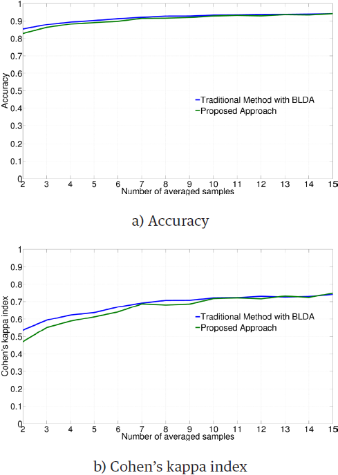
Table 4 Averaged metrics by subject, for BLDA.
| Subject | Traditional Approach | Proposed Method | ||
| Accuracy | Kappa | Accuracy | Kappa | |
| 1 | 0.99 ± 0.08 | 0.95 ± 0.33 | 0.98 ± 0.08 | 0.94 ± 0.33 |
| 2 | 0.96 ± 0.09 | 0.87 ± 0.30 | 0.95 ± 0.09 | 0.85 ± 0.30 |
| 3 | 0.86 ± 0.12 | 0.30 ± 0.25 | 0.86 ± 0.12 | 0.33 ± 0.26 |
| 4 | 0.95 ± 0.10 | 0.82 ± 0.30 | 0.95 ± 0.10 | 0.79 ± 0.30 |
| 5 | 0.98 ± 0.07 | 0.94 ± 0.31 | 0.98 ± 0.10 | 0.92 ± 0.30 |
| 6 | 0.86 ± 0.12 | 0.58 ± 0.27 | 0.84 ± 0.13 | 0.53 ± 0.27 |
| 7 | 0.88 ± 0.12 | 0.48 ± 0.28 | 0.87 ± 0.12 | 0.49 ± 0.28 |
| 8 | 0.90 ± 0.11 | 0.67 ± 0.28 | 0.88 ± 0.12 | 0.62 ± 0.28 |
| 9 | 0.95 ± 0.09 | 0.86 ± 0.30 | 0.94 ± 0.10 | 0.82 ± 0.29 |
| 10 | 0.95 ± 0.10 | 0.79 ± 0.30 | 0.94 ± 0.10 | 0.78 ± 0.30 |
| 11 | 0.95 ± 0.09 | 0.83 ± 0.30 | 0.94 ± 0.10 | 0.80 ± 0.29 |
| 12 | 0.89 ± 0.12 | 0.43 ± 0.27 | 0.89 ± 0.12 | 0.45 ± 0.27 |
| 13 | 0.85 ± 0.12 | 0.58 ± 0.27 | 0.82 ± 0.13 | 0.52 ± 0.26 |
| 14 | 0.89 ± 0.12 | 0.46 ± 0.28 | 0.88 ± 0.12 | 0.46 ± 0.28 |
| Average | 0.92 ± 0.29 | 0.68 ± 0.11 | 0.91 ± 0.29 | 0.66 ± 0.11 |
*The difference is highly significant, with a Student’s t-test (p < 0.01).
Number of samples: 372 for subject 1,504 for the rest.
Discussion
Results of LSVM and logistic regression are similar. When we trained the classifiers with the traditional approach, Cohen's kappa index decreased as the number of averaged samples was increased in the testing samples. The observed decrement of kappa is due to the probability of classifying by chance pe , as defined in Equation (3). The value of pe increases with the increase in the number of averaged samples. Meanwhile, the accuracy only has little changes when the number of averaged samples by trial is increased. As a consequence, pe is closer to the accuracy as the number of averaged samples is greater, so kappa is decreased.
Tables 3 and 4 indicate that subjects 3, 4, 6, 7, 8, 12 and 14 have averaged kappa values close to or lower than 0.05. It is a strong indicator of the presence of the accuracy paradox in these cases. It is an indication that discriminative classifiers try to label most of the samples as non-P300 targets in the traditional approach because in the P300 speller, there are more non-P300 samples than P300 ones. In addition, since each discriminative classifier is trained in single trials, it learns features that averaged trials do not have, because of the different statistical properties of single and averaged data. As a consequence, most of non-P300 features will be learned in this case.
By contrast, when we trained the classifier with the proposed method, the performance improved significantly. The improvement of kappa indicates that the classifiers learn features from both P300 and non-P300 classes. This is because the accuracy gets greater values than pe when the number of averaged samples by trial is increased. Consequently, the accuracy, and thus kappa, will be higher, as seen in Figures 1 and 2. The reasons for this are balanced data, similar statistical properties for training and test samples, and more statistical variation by class due to an increase in sample size. Here, it is necessary to remark that the inconvenience of using unbalanced classes with single trials for training discriminative classifiers is due to the difference in statistical properties of the data used for testing the classifier. Again, the advantage of training with re-sampled and averaged samples is statistically significant.
By contrast, although results of stepwise and Bayesian LDA were similar between them, they are different from the discriminative classifiers. ANOVA tests give significant differences in the methods, whereas the Student’s t-test does not reject the statistical equality of the results, as presented in Tables 5 and 6. The discrepancy of the statistics is due to the origin of the standard deviation in each test. The Student’s test employs weighted pooling of the variances, whereas ANOVA uses the mean square of the error from the data. Thus, the standard deviation by subject lies between 0,07 and 0,13 for accuracy and between 0,25 and 0,33 for kappa, the mean square errors are around 0,0006 for accuracy and 0,006 for kappa. This means that the differences of magnitude between standard deviations are around 183 for accuracy and 48 for Cohen’s kappa index. Therefore, with the same averaged metrics, both types of tests give different results: ANOVA sees a gap between the levels of the design variable, whereas the Student’s t-test gives small values of the statistics.
Another issue worth considering is the nature of the LDA-based classifiers. They try to fit the data to a set of Gaussian models, with a mean by class and a common covariance matrix [25]. When new data are presented to the classifier, they are compared with each model. Later, a class is assigned to the data when the highest score or probability value is obtained from the corresponding model of the set. This score or probability comes from the distance between the data and each mean. In our study, both classifiers map the data to a score value, according to a model of regression before the generation of Gaussian models. This means that the models are also scalar rather than multivariate, unlike discriminative classifiers, where the mapping to the class is direct [25]. Consequently, discriminative models are more affected by the statistical nature of the data. This is reflected in the difference of the results between generative and discriminative classifiers.
Conclusions
In this study, a bootstrapping method is presented to solve two important problems in the P300 speller. The method generates a new training set by re-sampling with replacement from the original set, reaching two important goals at the same time.
First, the number of trials across classes is balanced. It avoids dropping data in the process, as suggested in other approaches [13] [14] [15] [16] [17], which prevents a possible bias in the classification results.
Second, the statistical properties of the training data are made equivalent between the training and the test sets. This is achieved when the number of averaged trials for each instance in training equals the number of averaged samples during testing.
Unbalanced classes and the difference in statistical properties are considerable issues present in the state-of-the-art implementations of the P300 classification task.
Results presented here indicate that the proposed method improves significantly the detection of P300 and non-P300 classes in linear discriminative classifiers, by dealing with the aforementioned issues.

