


 text new page (beta)
 English (pdf)
 Article in xml format
 Article references
 Send this article by e-mail
 Cited by SciELO
  Similars in
SciELO
Similars in
SciELO 
 Permalink
INTRODUCTION
The immobilization of joints by a splint for a fracture’s restoration or the lack of movement in the joints caused by a disease such as hemiplegia, will result in complications such as joint stiffness, muscle atrophy, pain and edema. Rehabilitation is accomplished through therapeutic exercises. According to the APTA (American Physical Therapy Association) therapeutic exercise is the systematic implementation of planned physical movements, postures, or activities designed to: 1) remedy or prevent impairments, 2) enhance function and 3) enhance fitness and well-being. A rehabilitation program may include a range of different types of exercises to prevent aerobic capacity deterioration, or to improve muscle strength, power and endurance, flexibility or range of motion, coordination, balance and agility. The physiotherapist is the specialist in charge of dealing with all the consequences of injuries and achieve the best recovery in the shortest possible time [2].
Exoskeletons are mechanical structures of support, equipped with a variety of electronic sensors and actuators. They are mechatronic devices with two main objectives: The first objective is the enhancement of the strength and resistance of the human body, beyond his natural capacities. The second objective is to provide a useful tool in the task of rehabilitation. The assistance of the physiotherapist for helping a patient exercise can vary depending on the desired task. Indeed we have different cases: a) the patient can be completely attended by the physiotherapist, b) the patient may be partially helped by the physiotherapist or c) the patient can exercise alone. There are different types of rehabilitation exercises. For instance, strengthening exercises are used to increase the amount of force of a muscle. There exist also isokinetic exercises which vary the resistance while maintaining a constant rate of motion [3].
Stationary systems are those robotic mechanisms designed to exercise the human ankle and knee motions without walking. The patient is positioned always in the same place, and only the target limb is exercised. The Rutgers Ankle was the first of this kind.
A more recent system, the Active Knee Rehabilitation Orthotic Devices (AKROD), provides variable damping at the knee joint, controlled in ways that can facilitate motor recovery in poststroke and other neurological disease patients and to accelerate recovery in knee injury patients. This configuration is similar to LItio however it is only for knee [4].
The Northeastern University Virtual Ankle and Balance Trainer (NUVABAT) rehabilitation system is a low cost, compact, mechatronic rehabilitation device for training the ankle Range Of Motion (ROM) exercise in sitting and standing positions and also weight lifting and balance training in standing position [5]. The Department of Mechanical Engineering at the King’s College has proposed an ankle rehabilitation robot based on a parallel mechanism with a central structure [6], a disadvantage of this type of designs is that being fixed to eart does not allow an autonomy. The University of Auckland has also developed a parallel robot to perform ankle rehabilitation exercises [7]. In this last system, the human ankle is secured to the end effector in such a way that it produces kinematic constraint of the robot. The IIT (Istituto Italiano di Tecnologia) has developed a high performance ankle rehabilitation robot [8], device allows plantar, dorsiflexion, inversion and eversion using an improved performance parallel mechanism that makes use of actuation redundancy to eliminate singularity and greatly enhance the workspace dexterity. A disadvantage of this 3 types of designs is that being fixed to eart does not allow an autonomy.
This paper describes the design, control and performance of the ELLTIO prototype for knee and ankle rehabilitation, using SEA actuator to perform a tracking trajectory on each joint, from two desired paths proposed using the real recorded data during a rehabilitation exercise, as reference. We use the ELLTIO as an "Active Foot Orthosis" (see Figure 1), to make rehabilitation routines in a volunteer diagnosed with Left Hemiparetic Infantile Cerebral Palsy. A professional therapist made a passive rehabilitation routine appropriate for the patient. A motion capture prototype is used to record the angular position and velocity in human joints. Such information is used to generate a sine function with the same amplitude and frequency used by the therapist during the routine. The obtained trajectory is programmed into the microcontroller of the exoskeleton which should reproduce the movement as accurately as possible. The user performs the rehabilitation exercise during a period determined by the therapist and then verifies the progress of the patient improvement. The therapist could change the frequency and the amplitude of the routine depending on the patient rehabilitation progress and apply with the exoskeleton a new routine forming a cycle. To control the exoskeleton we use an adaptive control. This method of controlling the exoskeleton allows adaptation to unknown parameters of the patient who may be changing as time passes such as mass and limb length. Furthermore, in order to use the exoskeleton in different patients, the chance in mass and length of the limbs from one user to another should be taken into account. Therefore, the parameters estimation is an important part of the strategy.
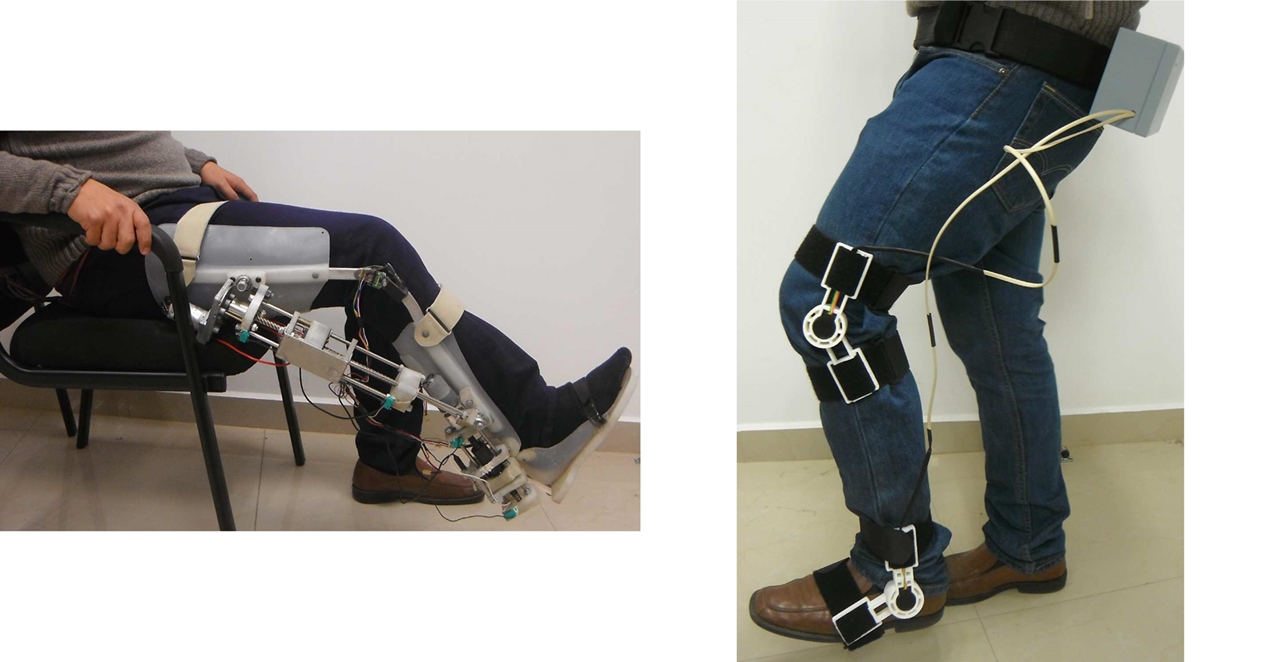
FIGURE 1 The ELLTIO prototype with two degrees of freedom and the motion capture prorotype for knee and ankle.
The advantages of performing a rehabilitation routine using an exoskeleton is that the angular position, the velocity, the resistance or opposing force can be increased gradually with precision when repeating an exercise sequence. Exoskeletons in collaboration with a therapist will execute such tasks more accurately.
The exoskeleton was tested with the help of a physiotherapist and a volunteer. The volunteer was a child of 14 years old and his body parameters are given in Table 1. He was diagnosed with Left Hemiparetic Infantile Cerebral Palsy. This kind of disease affects one side of the body, reducing motor skills due to the spasticity. Also different body functions can be affected and produce learning disabilities, hearing impairment, ophthalmologic abnormalities (strabismus), loss of using or understanding speech and muscle tone. For this reason the therapist suggested some exercises, to improve learning, coordination and muscle tone.

The paper is organized as follows: Section II presents the dynamical model of the exoskeleton.
The control scheme is given in section III. The design and description of the prototype is detailed in section IV. Section V describes the numerical results and the performance of the proposed approach. The experimental results are shown in section VI. Finally the concluding remarks are given in section VII.
DYNAMICAL MODEL
Mechanical Structure
ELLTIO is a planar robot with two degrees of freedom, the movement of the joints is restricted to the sagittal plane (Figure 2).To obtain the mathematical model we used the Euler - Lagrange approach. This mechanical prototype is used for flexion and extension of the knee and the ankle. The joint angle are limited to: q 1 ∈ [0, 60] degrees and q 2 ∈ [−14, 2] degrees, to avoid exceeding the patient comfort angles. The links of the exoskeleton are rigid with mass m 1 for the lower leg and m 2 for the foot, and their lengths are l 1 and l 2 respectively with center of mass in l C1 and l C2 , respectively. Finally, I 1 and I 2 denote the moments of inertia of the links with respect to the axes that pass through the respective centers of mass and are perpendicular to the plane x − y (see Figure 2).

We consider that:
where m 1Body and m 2Body represent 4,6% and 1,4%, of the total mass of the user respectively [9], the m 1Exo and m 2Exo are the masses of the links of the exoskeleton. Therefore the model for ELLTIO is:
Where
The torque produced by the human in the knee is τhk= 0 and the human ankle is τha= 0 because it is a passive exercise that represents a complete dependence of the exoskeleton without human effort. The relation between the forces of the actuators (ƒa1, ƒa2) and the torques produced by the exoskeleton on the ankle τ2 and the knee τ1 are given by:
Series Elastic Actuator
Series Elastic Actuators have been preferred in the experimental prototype because force control can be conveniently achieved [11] and [12]. The principle of operation is a compliant element (spring) which is introduced between the gear train and the load. The force is estimated by using a position sensor and the Hook’s law (F= k s x). The main advantages of this approach are that it has inherent tolerance, low impedance and high force fidelity.
A graphic representation of the dynamic model for the SEA is shown in Figure 3. The motor produces a torque τ mot , through the transmission of gain K generating a force ƒ m . The transmission consists of a ballscrew, the coefficient friction between the nut and the ballscrew is b m , the nut has a relatively small mass mn with respect to the total mass of the load m l . The resultant force generated by the actuator is ƒ a . A spring is placed between the masses having a stiffness coefficient k s . Notice that the mass mn, the spring stiffness k s and the friction bm are opposed to the action of ƒ m , which can be represented by a second order differential Equation as follows:
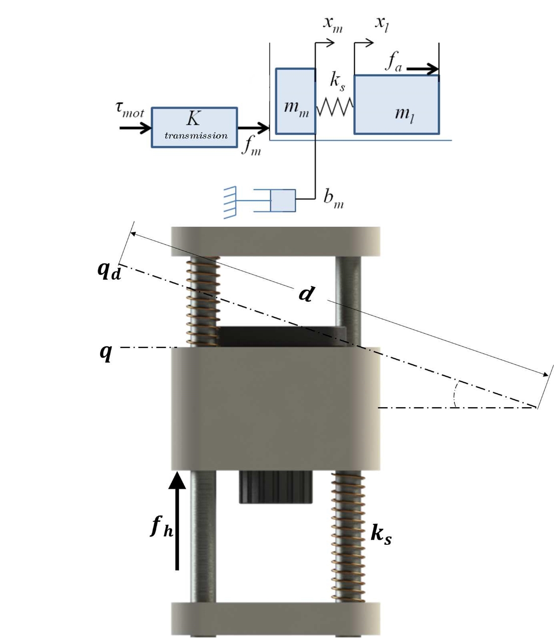
The position of the nut and the load are represented by xm and xl respectively. We can see that ƒ
a
is defined as
From (4) and (5) we obtain the dynamic model of the actuator:
Coupling Dynamic Models
Equation (6) is valid for both SEA 1 and SEA 2 actuators. In the sequel we will refer to the knee actuator with the lower index i= 1 and i= 2 for the ankle actuator (See Figure 2). Combining the dynamic model (2) and (6) and using the change of variables, z 1 = ƒ a and z 2 = ƒ a , we can rewrite the dynamic of the actuator as follows:
Where
Similarly, the dynamic model (2), can be expressed as:
Where
with
Equation (10) has k isolated roots, i.e.,
We suppress the lower index j because the system has only one root in
The singular perturbation approach can be applied in our system since it satisfies the conditions of Thiko ov’s theorem [13 ]. Therefore introducing (12) into (3) we obtain the new inputs:
with
METHODOLOGY
PD Control with Adaptive Compensation
In this section we will introduce a PD control law with adaptive compensation, that will be used to follow the proposed computer generated trajectories to accomplish the desired rehabilitation exercises routines [14]. The patient size who will use the prototype is constrained to 1,65 m height. But even with such restriction, the weight of each user is different and therefore it is essential that the system has the ability to adjust its parameters to properly adapt to each user. The model of the exoskeleton (2), can be rewritten as the product of a vector function Φ which contains nonlinear terms of the state (the generalized coordinates and its derivatives) and the vector of dynamic parameters Ɵ. This property is commonly known as "linearity in the parameters", which is formally stated bellow.
Property 1. "Linearity in the dynamic parameters": For the matrices M(q, Ɵ), and C(q, q̇ , Ɵ) and the vector G(q, Ɵ) we have the following:
for all
where k a (q, u, v, w) is a vector of n × 1, Φ(q, u, v, w) is a matrix of n × m and the vector Ɵ ∈ ℜ m depends only on the dynamic parameters of the manipulator and its payload.
We can rewrite Equation (2) as:
and defined as:
and
where q̃ = q
d − q is the position error and is defined as
where
with
and
On the other hand, according to the parametrization, given a vector
Taking (16) into account, we propose the following control law:
where, K
p
, K
v
are symmetric positive definite gain matrices,
where
Equilibrium Point
Before proceeding to obtain the closed-loop Equation we first write the parametric error vector
From the above expression, the control law (17) takes the following form:
Using the control law expressed above and substituting the control action into the Equation of the robot model (2), we get
On the other hand, since the vector of dynamic parameters have been assumed constant then
The closed-loop Equation, which is obtained from (21) and (22), may be written as
which is a nonautonomous differential Equation and the origin of the state space
is an equilibrium point.
Stability Analysis
The stability analysis of the origin of the state space for the closed-loop system is carried out using the following Lyapunov function candidate:
The time derivative of the Lyapunov function candidate becomes
Developing the first term in the last Equation it follows:
Solving for
and substituting into (27), we obtain
Using the following property that established a relationship between the inertia matrix M(q) and the Coriolis matrix C(q̇, q):
and substituting into (27), we obtain
Now, using
which can also be expressed as
After some further simplifications, the time derivative
The terms
Solving for
where
Property 1. Consider a continuously differentiable function ƒ : R+ → Rn which satisfies
Then, the function f, necessarily satisfies:
Since
Using the theorem of Rayleigh−Ritz [16], we have:
Integrating the inequality from t = 0 to t = ∞ that is
where we defined
The integral on the left-hand side of this inequality is calculated to obtain
We recall that the Lyapunov function candidate:
is positive definite, radially unbounded and decrescent and moreover, all the signals are bounded. Therefore,
From this expression we immediately conclude that
where the left-hand side of the inequality is finite positive and constant. This means that the position error q̃ belongs to the
DESCRIPTION OF THE ELLTIO PROTOTYPE
The main structure of ELLTIO prototype consists in a commercial quadrilateral orthopedic orthosis for the right leg which is manufactured in polypropylene with parallel duralumin bars as structural support; a very commonly material in this kind of devices.
The prototype length is about 88 cm and was instrumented with SEA actuators, these linear actuators transform the torque generated by a motor τ
mot in a linear force ƒ
a
. The first actuator produces a torque τ
1
in the joint q
1
, due to the force
We used an optical encoder 600EN-128-CBL for measuring the angular position q for each joint and a gyroscopic sensor LPR510AL for measuring the angular velocity q̇. Using Hooke’s law
We can distinguish the following three cases, i) ƒ h = 0 which implies q d = q and means the intention of the human to maintain the position. ii) fh > 0 which implies q d > q and means the intention of the human to extend the leg. iii) fh < 0 which implies q d < q and means the intention of human to flex the leg.
The output signals from the sensors were processing using the Rabbit 3400 microcontroller. The knee and ankle joints use a SEA to generated the exoskeleton force ƒm. Each joint was designed to satisfy the angular position limit and using the same main components. An MD03 driver was used to control a DC motor with torque τ mot and coupled through a gear box to the base of a ball screw. As the ball screw turns it produces a linear displacement on the nut which generates the torque inputs for each joint. A graphical representation of the components of the ELLTIO prototype is shown in the left side of the Figure 4.

MOTION CAPTURE SYSTEM FOR LOWER LIMBS
The main goal of this work is perform exercise routines for the right leg’s knee and ankle rehabilitation using ELLTIO exoskeleton, in very important clarify that the exoskeleton is can be used as a tool for the rehabilitation task, and not as a new rehabilitation technique. For this reason we design and construct a unexpensive motion capture prototype for the lower limbs, to measure the angular motion for hip, knee and ankle displayed in real time, through the legs motion of a 3D dummy, using MATLAB. The main parts of the prototype were built using a 3D printer, an incremental encoder was used to measure the angles and a wireless connection was implemented using an Xbee to send the obtained data to a PC for storage, see the rigth side of the Figure 4.
Now, to generate the desired trajectories we use the following methodology (See Figure 5): First a certificated physiotherapist performs a rehabilitation routine, with a volunteer diagnosed with a kind of motion disability. Second the physiotherapist defines the correct amplitude, frequency and motion range for each joint, in this case for the knee and ankle. Third, we use the motion capture system weared by the volunteer and we store the angular trajectories. Fourth the obtained data is analyzed to identify the corresponding parameters and then reproduce them through the exoskeleton. Finally the obtained desired trajectory is programmed into the exoskeleton’s PC and we perform the same routine while the physiotherapist is only monitoring the evolution of the exoskeleton.

Application Case
A physiotherapist proposes a rehabilitation routine tested in an healthy adult but based in a person with the body parameters given in Table 1. and diagnosed with Left Hemiparetic Infantile Cerebral Palsy. This kind of disease affects one side of the body, reducing motor skills due the spasticity. Also, different body functions can be affected so that the patient may present learning disabilities, hearing deficits, ophthalmologic abnormalities (strabismus), loss of using or understanding speech and muscle tone. For this reason the therapist suggested the following exercises, to improve learning, coordination and muscle tone.
Sitting on a high surface (table, bench) the human extends the leg and hold it for 15 seconds. Perform 3 sets of 15 repetitions and resting 30 seconds between each set. Perform 3 times the routine and rest 30 seconds between each. The exercise is shown in Figure 6a.
Standing up, with legs apart at hip level, flex the leg in parallel to the ground (90). Perform 3 set of 20 seconds each one and resting 10 seconds between each set. Perform 3 times the routine and rest 30 seconds between each. The exercise is shown in Figure 6b.

Then, following the proposed methodology, we recorded the pattern for the right leg to obtain and generate the desired trajectories for the knee and ankle. The trajectories were generated using the following functions:
The values for the exercise 1 are

FIGURE 7 Recorded trajectories for knee and ankle joints during the exercises performed by the volunteer with the help of the physiotherapist (dashed blue line) and the proposed computer generated trajectories that will be perform by the patient with the help of the exoskeleton (red line). The data from the exercise 1 appear at the left and the right for exercise 2.
RESULTS AND DISCUSSION
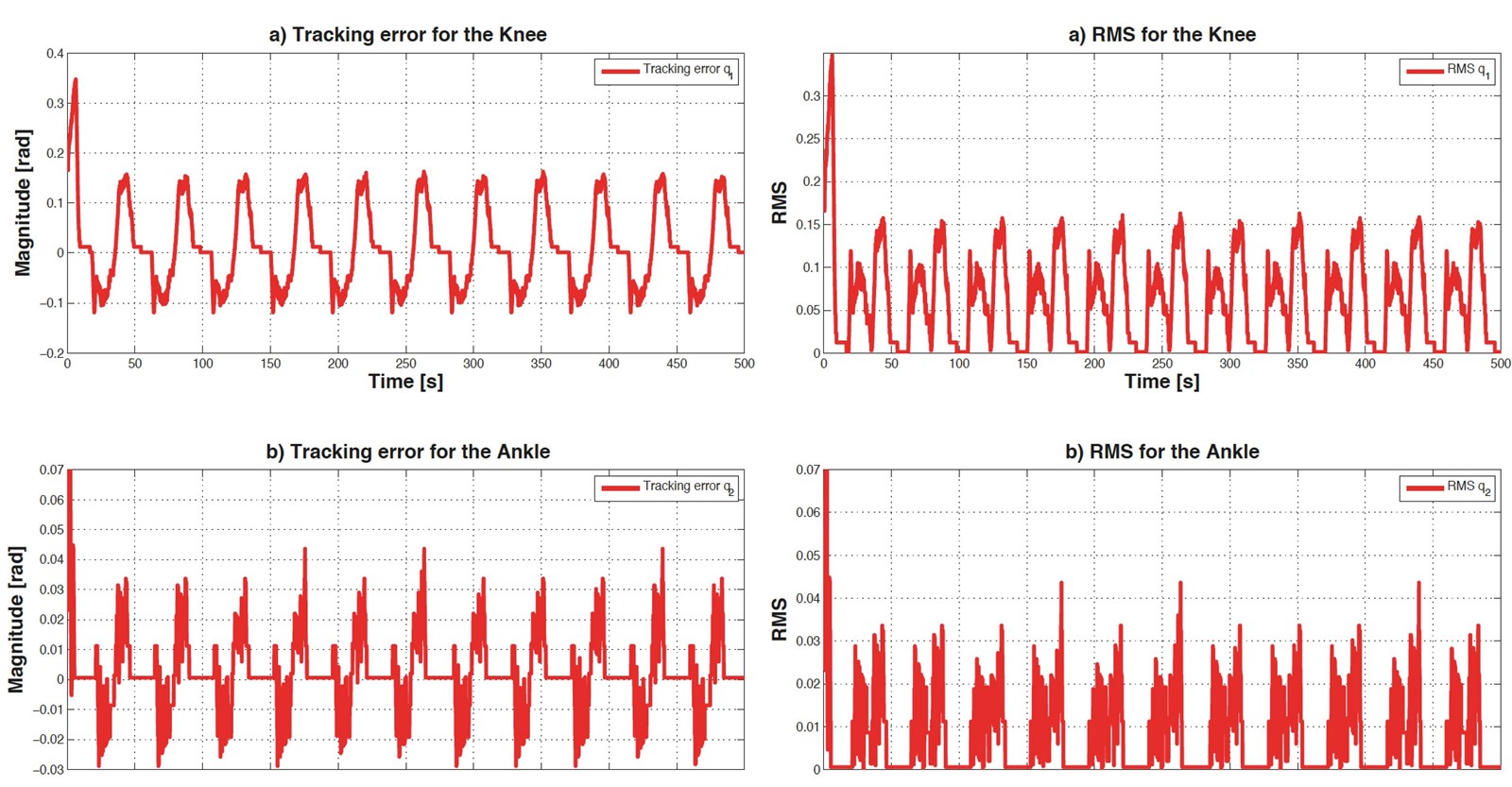
The exoskeleton was programmed to perform therehabilitation exercises using a PD control with adaptive compensation assuming that the system parameters are unknown. The control objective is to track the desired trajectory in real-time and estimate the parameters of the system while the exercise is being executed.
The left side of Figure 8 shows the experimental tracking trajectory for the joints angles (Knee and ankle). The routine that was generated by the physiotherapist and programmed in the exoskeleton shown by the dotted line, while the trajectory generated by the exoskeleton measured by the encoder in real time is shown in full line. As can be observed, they are very similar.

FIGURE 8 Tracking trajectories’ results for knee joint (q1) and ankle joint (q2) along the experimental test performed by the exoskeleton for the exercise 1 (left) and the same exercise when we duplicated the frequency (right).
We double the frequency value in exercise 1 and can note that the exoskeleton can also follow the desired trajectory (see the rigth side of Figure 8). Therefore we can reduce the amount of time needed by a physiotherapist to implement a new routine. The trajectories pro grammed in the Microcontroller may also serve as persistent perturbation that is needed in the adaptive control law to improve parameters estimation. Programming the adaptation law (18) in the microcontroller we obtained the estimation of the system parameters
CONCLUSIONS
This paper has presented a prototype of the exoskeleton ELLTIO designed for rehabilitating knees and ankles using a passive rehabilitation routine. The experimental prototype is controlled using a PD control law with an adaptive compensation algorithm. The unknown parameters are identified online so that the two joint angular positions track the corresponding desired trajectories. The prototype and the control strategy have been successfully tested in real-time experiments. The mass of one of the links (lower leg) has been changed and it has been observed that the knee and ankle joints were able to track the predefined trajectories after some transient period. Therefore, it has been shown that it is possible to use the same exoskeleton on patients having different weights.
For patient safety, besides the program containing the microcontroller, the exoskeleton has mechanical brakes that prevent exceeding the comfort angles. For security, the exoskeleton has an emergency stop in place. Furthermore, the speed and acceleration of the articulations are limited by software and by mechanically. Moreover, a therapist generated the real routine adapted for the child with muscular dystrophy. This routine was used in the experiments presented in this paper which were obtained for a healthy adult. Future work includes implementing the proposed approach to estimate the motion capabilities for the user’s limbs using the proposed identification algorithm to obtain the best rehabilitation results.

