


 text new page (beta)
 English (pdf)
 Article in xml format
 Article references
 Send this article by e-mail
 Cited by SciELO
  Similars in
SciELO
Similars in
SciELO 
 Permalink
INTRODUCTION
The California sardine (Sardinops sagax, Jenyns 1842), locally known as sardina Monterrey, is a temperate species distributed from the Gulf of California to Kamchatka, Alaska (Miller & Lea, 1972) and is part of the small pelagic fish. It is generally considered to be isolated in the Gulf of California from other subpopulations (Lluch-Belda & Magallon, 1986), and it is found principally in the Gulf central region (Hammann et al., 1988). In the Gulf of California, estimates of California sardine abundance, as well as biomass, have shown great variability. Recruits number increased from the early seventies to a peak in the mid-eighties, falling to very low levels between 1990 and 1992, and again an upward trend with high variability until reaching a historical maximum in 2007 (INAPESCA, 2012).
Small pelagic is one of the main fishing resources around the world. In Mexico, it is the main fishing resource in terms of volume, sometimes representing up to 30% of the total annual catch in the country (INAPESCA, 2012; INAPESCA, 2018). Catch species composition varies, being the California sardine the most representative with 38% of catch (SADER, 2019). The sardine fishery moves south and north as these fish populations migrate south in the winter and spring, and north in the later spring and summer. The Mexican small pelagic fishery operates in the central gulf and, to a much smaller extent, along the west coast of southern Baja California (Lluch-Belda & Magallon, 1986).
This fishing resource is an important source of quality protein for human consumption. The industry uses it as raw material for the production of balanced feed for poultry, swine, and aquaculture. The commercial (industrial and artisanal) and sport fishing use it as bait. Besides, this fishery is an important source of employment (Gómez-Muñoz et al., 1991; Cisneros-Mata et al., 1995; Lluch-Belda et al., 1996); it generates around 5,000 direct jobs and a similar amount of indirect jobs (INAPESCA, 2012).
Currently, the fleet consists of boats from 23 to 35 meters in length and 101 to 285 metric tons of hold capacity (SADER, 2019). Presently, 48 vessels operate in the Gulf of California. The fishery uses a purse seine net with an average mesh size of 25 mm. Seine length varies between 366 and 640 m, and seine height varies between 40 and 100 m. All boats have hydroacoustic equipment for the location of fish schools. For fleet operations, a 40 NM radius of action has been established from the base port (Rodriguez et al. 1996). The fleet operates from two main ports (Mazatlán and Guaymas) and within several fishing zones in the Gulf of California (Figure 1).
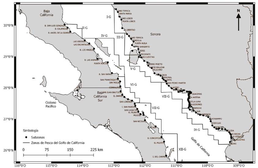
Figure 1 Fishing zones where the small pelagic fishery operates in the Gulf of California (modified from Jacob et. al, 2018).
The NOM-003-SAG/PESC-2018 regulates the small pelagic fishery with a minimum size for the California sardine of 150 mm of standard length (SADER, 2019). The standard also establishes the maximum volume of fishes caught below the minimum size being 20% of the total catch. Besides, the standard also defines boat characteristics, gear characteristics, and three fishing regions. It also suggests admitting on-board observers in 20-30% of trips for gathering information on fishing operations, species composition, bycatch, and ETP species catch.
According to the National fisheries chart (INAPESCA, 2018), the fishery is exploited at the maximum sustainable yield. In July 2011, the Marine Stewardship Council (MSC) certified as sustainable and well managed the 36 vessels fleet of the small pelagic fishery in the Gulf of California with the California sardine as target species and the purse seine as fishing gear. Keeping the MSC certification is of great importance for managers and the industry; therefore, during the 2016-2018 period, an onboard Observer Program collected important data during fishing operations, including biological and fishery information. However, preliminary results indicate that the fishery might be catching small organisms that could produce growth overfishing. In this paper, we used the onboard Observer Program data for the estimation of the percentage of organisms below the minimum size and for determining the potential variables affecting the sardine´s size caught by the fishery, in an attempt to establish management measures that contribute to avoid growth overfishing and assure the sustainable exploitation of this fishing resource.
MATERIAL AND METHODS
Observer Programs are an important tool for gathering information for fisheries management. In particular, the small pelagic fishery in the Gulf of California had an Observer Program between 2016 and 2018 observers following a monitoring protocol (Jacob et al. 2018; Hernández & Jurado, 2018).
Onboard observers took biological samples within the fishing operation zones in the Gulf of California (Fig. 1) during the 2017 and 2018 seasons using random stratified sampling. In 2017, biological samples came from 20 boats, the following year, samples came from 29 boats. Observers registered biological, physical, and technological variables. With those data, we carried out a data exploratory analysis. We analyzed seasonal size variation and the interannual size variation using the Kruskal-Wallis and the Wilcoxon’s signed-rank test respectively. For the post hoc test we used the function posthoc.kruskal.nemenyi.test implemented in the R package. We also explored the size variation by mesh size (Kruskal-Wallis test), by Boat, and by Zone. Later, we investigated the potential predictor variables affecting the sardine´s size caught by the purse seine fishery through analysis of correlation and covariance ANCOVA. For the maximal ANCOVA model, we defined the continuous response variable as the standard length. Continuous covariates included mesh size (MS), depth (D), latitude (Lat), longitude (Lon), seine length (SL), and the sein height (SH). On the other hand, factors included year (Y), month (M), maturity (MA), Sex (Sex), fishing zone (Z), and boat (B). We included in the model first-level interactions and a normally distributed error (ε):
L = β0 + β1 M + β2 Y + β3 MS + β4 D + β5 Lat + β6 Long + β7 Sex + β8 MA + β 9 Z + β10 B + β11 SL + β12 SH + first level interactions + ε (1)
We set up the model using the function lm from the statistical package R (R core team 2018). The factor levels are shown below (Table 1). The model simplification process was done initially using the step function from the same statistical package. Later, we applied a manual stepwise process; in each step, we deleted a no significant term and applied ANOVA for the current model and the updated model (Crawley, 2007). The model simplification was justified if it caused a negligible reduction in the explanatory power of the model (p > 0.05). We repeated this procedure until all terms included in the model were significant; the resulting model was considered as the minimal and adequate model. Finally, we applied ANOVA to the minimum model to find out the amount of variability explained by each predictor variable.
Table 1 Factor levels used in the ANCOVA model (1) to assess the potential drivers of the caught sardine´s length in the Gulf of California.
| Year | Maturity | Fishing zone | Boat | Month |
| 2017 | 1 | I-G | 1 | 1 |
| 2018 | 2 | II-G | 2 | 2 |
| 3 | III-G | 3 | 3 | |
| 4 | IV-G | 4 | 4 | |
| 5 | V-G | 5 | 5 | |
| VI-G | 6 | 6 | ||
| VII-G | 7 | 7 | ||
| VIII-G | 8 | 8 | ||
| IX-G | 9 | 9 | ||
| 10 | 10 | |||
| 11 | 11 | |||
| 12 | 12 | |||
| 13 |
RESULTS
The number of samples collected by the Onboard Observers Program distributed in each operating zone were: Zone I-G (615), Zone II-G (79), Zone III-G (1244), Zone IV-G (1219), Zone V-G (2379), Zone VI-G (514), Zone VII-G (504), Zone VIII-G (299), Zone IX-G (1730).
Regarding the size structure, the Observer Program´s data suggest that the California sardine standard length in the Gulf of California ranged from 64 mm to 230 mm, the average length was 158.6 ± 19.8 mm, with a median of 160 mm. The standard length distribution is shown below (Figs. 2a and 2b); there are some outliers mainly in the lower end of the distribution (Fig. 2b). The distribution of the sardine´s length is not normal (p-value = 2.2x10⁻¹⁶). Although the estimated mean is greater than the minimum size (150 mm) established in the regulation (SADER, 2019), results suggest that 32.9% of the organisms caught are below the minimum size (Fig. 3), 12.9% above the established tolerance limit (20%).
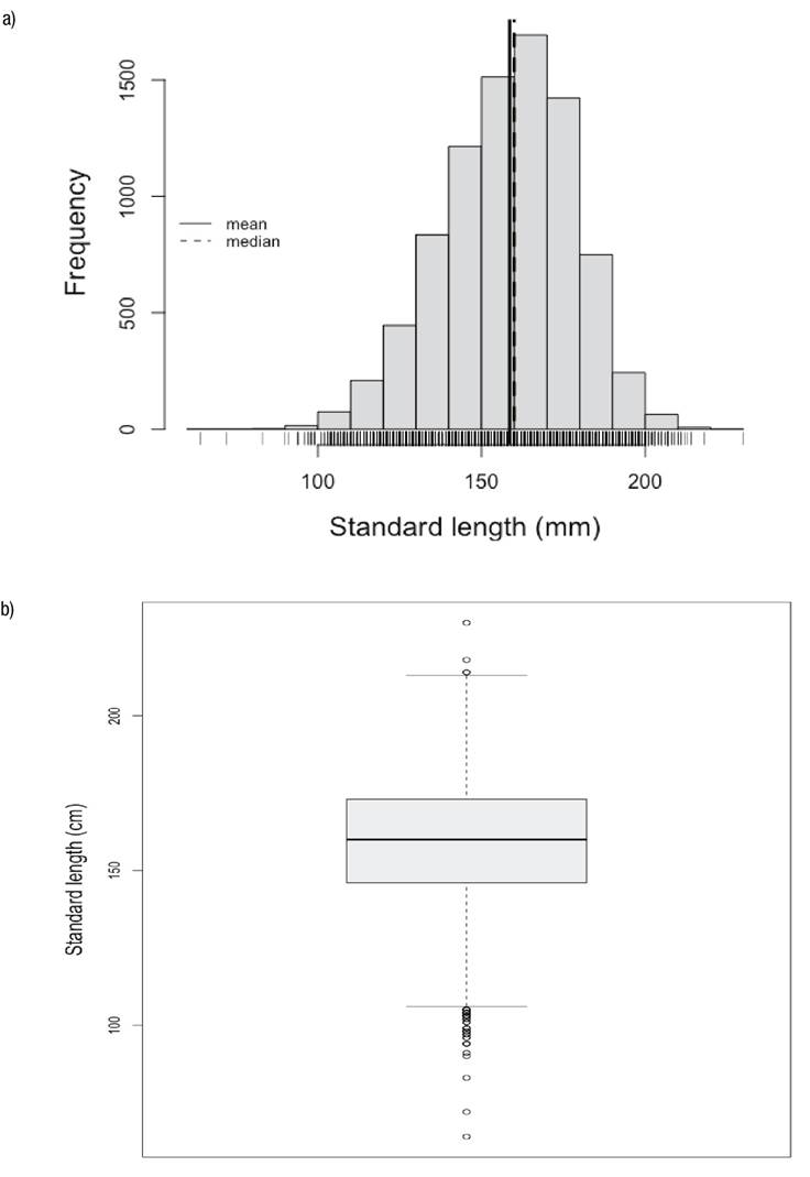
Figure 2 a) California sardine standard length distribution for 2017-2018 in the Gulf of California, b) Boxplot for the sardine standard length.
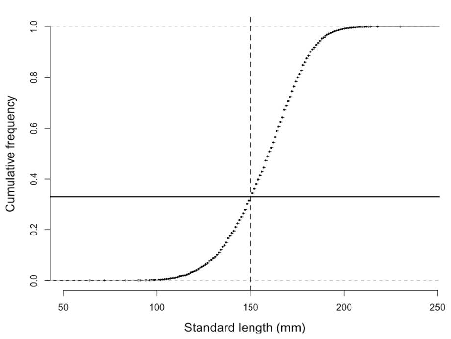
Figure 3 Cumulative distribution of the sardine´s standard length caught by the small pelagic fishery in the Gulf of California.
On regard to the seasonal variation (Fig. 4), results suggest the lower standard length values occurred during June (142.8 ± 18.9 mm) and July (135.9 ± 19.0 mm), while the highest values occur in March (170.6 ± 16.1 mm) and April (170.8 ± 9.4). The Kruskal-Wallis rank sum test suggested that means are not all equal (p-value < 2.2x10⁻¹⁶). Results from the post hoc test also suggested that the monthly means for March and April are statistically the same (Pr(>||) = 1.0). Likewise, the mean for February is statistically equal to the means from March and April (Table 2), and the mean of January is statistically equal to the means from November (Pr(>||) =0.34) and December (Pr(>||) =0.24). The remaining mean comparations are statistically different (Table 2).
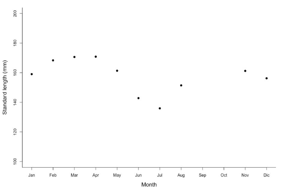
Figure 4 Monthly variation of sardine´s standard length caught by the small pelagic fishery in the Gulf of California.
Table 2 Results from the post hoc Kruskal-Wallis test for the sardine´s standard length monthly average in the Gulf of California
| Month | 1 | 2 | 3 | 4 | 5 | 6 | 7 | 10 | 11 |
| 2 | 9.2x10⁻¹⁴ | ||||||||
| 3 | 0 | 0.18 | |||||||
| 4 | 0 | 0.31 | 1 | ||||||
| 5 | 5.1x10-06 | 6.1x10⁻¹⁰ | 1.2x10⁻¹³ | 1.1x10⁻¹³ | |||||
| 6 | 0 | 0 | 0 | 0 | 0 | ||||
| 7 | 0 | 0 | 0 | 0 | 0 | 3.2x10-07 | |||
| 10 | 2.3x10-09 | 0 | 0 | 0 | 1.3x10⁻¹⁴ | 3.1x10-04 | 9.7x10⁻¹⁴ | ||
| 11 | 0.34 | 0 | 0 | 0 | 4.4x10-04 | 0 | 0 | 9.2x10⁻¹⁴ | |
| 12 | 0.24 | 6.2x10⁻¹⁴ | 0 | 0 | 9.4x10⁻¹⁰ | 1.4x10⁻¹³ | 0 | 0.04 | 1.9x10-04 |
Regarding the interannual variation, results from the Wilcoxon rank sum test suggest that the mean standard length from 2017 (148.3 ± 13.1 mm) is significantly smaller than the mean (162.9 ± 20.1 mm) from 2018 (p-value< 2.2x10⁻¹⁶).
We estimated the mean standard length by zone (Table 3), the largest mean corresponded to the zone VIII-G (174.9 ± 20.1 mm) while the smaller mean corresponded to the zone IV-G (142.5 ± 19.4 mm). It is important to mention that the mean standard length in all zones was larger than the minimum size established, except for the zone IV-G.
Table 3 Mean standard length and percentage of organisms below the minimum size for the sardine caught in the Gulf of California during 2017-2018.
| Zone | Standard length | % |
| I-G | 155.4±23.2 | 37.6% |
| II-G | 159.5±12.9 | 27.8% |
| III-G | 163.2± 22.9 | 19.8% |
| IV-G | 143.2± 19.0 | 72.1% |
| V-G | 158.9 ± 16.0 | 34.1% |
| VI-G | 155.2± 21.8 | 45.3% |
| VII-G | 163.3± 17.0 | 26.2% |
| VIII-G | 165.8± 20.4 | 23.4% |
| IX-G | 165.3± 14.4 | 11.4% |
On the other hand, the largest average standard length by mesh size corresponded to the mesh size of 1.2 inches, while the smallest coincided with the 0.5 inches and the 1.9 inches of mesh size (Table 4). The Kruskal-Wallis test suggested there was at least one mean that is different from the rest (p-value < 2.2x10⁻¹⁶). The post hoc analysis suggested that the means from the 1.9 and .5 inches are the statistically equal (Table 5). Likewise, the comparisons 1.0-1.27 inches, 1.27-1.4 inches, 1.27-2 inches, and the 1.4-1.9 had mean standard lengths statistically equal (Table 5). The remaining comparisons presented different means (Table 5).
Table 4 Average standard ha length (mm) by mesh size (inches) for the California sardine in the small pelagic fishery.
| Mesh size | 0.5 | 1 | 1.2 | 1.27 | 1.3 | 1.4 | 1.9 | 2 |
| Average standard length | 150.2 | 159.6 | 169.4 | 156.7 | 163.5 | 154.5 | 150.2 | 156.6 |
| Sample size | 385 | 3236 | 467 | 204 | 1575 | 1088 | 206 | 1153 |
Table 5 Results for the posthoc Kruskal-Wallis test for the California sardine standard length regarding mesh size.
| Comparison | Value | Pr(>| |) |
| 1 - 0.5 = 0 | 14.001 | 7.1942x10⁻¹⁴ |
| 1.2 - 0.5 = 0 | 21.813 | < 2.22x10⁻¹⁶ |
| 1.27 - 0.5 = 0 | 6.277 | 0.00024276 |
| 1.3 - 0.5 = 0 | 16.931 | < 2.22x10⁻¹⁶ |
| 1.4 - 0.5 = 0 | 5.630 | 0.00176400 |
| 1.9 - 0.5 = 0 | 0.003 | 1.0 |
| 2 - 0.5 = 0 | 8.771 | 1.5606x10-08 |
| 1.2 - 1 = 0 | 15.084 | 7.2053x10⁻¹⁴ |
| 1.27 - 1 = 0 | 2.917 | 0.43945205 |
| 1.3 - 1 = 0 | 6.762 | 4.7617x10-05 |
| 1.4 - 1 = 0 | 12.027 | 7.6161x10⁻¹⁴ |
| 1.9 - 1 = 0 | 8.600 | 3.3417x10-08 |
| 2 - 1 = 0 | 6.963 | 2.3371x10-05 |
| 1.27 - 1.2 = 0 | 11.394 | 1.2401x10⁻¹³ |
| 1.3 - 1.2 = 0 | 10.219 | 1.3972x10⁻¹¹ |
| 1.4 - 1.2 = 0 | 21.121 | < 2.22x10⁻¹⁶ |
| 1.9 - 1.2 = 0 | 15.374 | 7.6161x10⁻¹⁴ |
| 2 - 1.2 = 0 | 17.970 | < 2.22x10⁻¹⁶ |
| 1.3 - 1.27 = 0 | 5.620 | 0.00181195 |
| 1.4 - 1.27= 0 | 2.754 | 0.51786870 |
| 1.9 - 1.27= 0 | 4.902 | 0.01236371 |
| 2 - 1.27= 0 | 0.367 | 0.99999614 |
| 1.4 - 1.3 = 0 | 15.963 | 1.2434x10⁻¹⁴ |
| 1.9 - 1.3 = 0 | 10.743 | 9.0106x10⁻¹³ |
| 2 - 1.3 = 0 | 11.524 | 1.0658x10⁻¹³ |
| 1.9 - 1.4 = 0 | 3.658 | 0.16059034 |
| 2 - 1.4 = 0 | 4.321 | 0.04652954 |
| 2 - 1.9 = 0 | 5.677 | 0.00153530 |
We also estimated the percentage of California sardine below the minimum size by Zone-Month combination (Table 6). The Observer program did not cover all Zone-Month combinations. In general, the highest percentages corresponded to June and July, although some high values showed up for May and December (Table 6). The overall highest percentages corresponded to May-June in the Zone IX-G and December in zone IX-G. However, the Zone IV-G presented consistently higher percentages throughout the year (Fig. 1, Table 6) and the highest percentage by Zone (Table 3). Zone VI-G also presented high percentages during some months of the year (Table 6).
Table 6 Percentage of Monterrey sardines below the minimum size by Zone and Month in the Gulf of California; FC - fishing closure, Avg - average of percentage of sardine below the minimum size.
| I-G | II-G | III-G | IV-G | V-G | VI-G | VII-G | VIII-G | IX-G | Avg | |
| Jan | - | - | - | - | 43.4 | - | 29.5 | 0.0 | 24.3 | |
| Feb | - | - | - | - | - | - | 0.0 | 36.0 | 18.0 | |
| Mar | 8.1 | 27.9 | 0.0 | 50.0 | 0.0 | 0.0 | - | - | 0.3 | 12.3 |
| Apr | - | - | 0.6 | 0.0 | 0.0 | - | - | - | 0.0 | 0.2 |
| May | 98.4 | - | 10.2 | 50.0 | - | 0.0 | - | 0.0 | 100.0 | 43.1 |
| Jun | - | - | 74.0 | - | - | 79.5 | - | 71.4 | 100.0 | 81.2 |
| Jul | - | - | - | 91.8 | - | 91.7 | - | 0.0 | 61.2 | |
| Aug | FC | FC | FC | FC | FC | FC | FC | FC | FC | FC |
| Sep | FC | FC | FC | FC | FC | FC | FC | FC | FC | FC |
| Oct | - | - | - | - | 42.6 | - | - | - | 42.6 | |
| Nov | 6.2 | - | 18.5 | 65.8 | 50.0 | 45.5 | - | 13.7 | 14.7 | 30.6 |
| Dec | 0.0 | - | - | - | - | 100.0 | - | - | 10.5 | 36.8 |
Additionally, we calculated the mean standard length by boat (Table 7). Six boats had an average standard length below the minimum size established. Those boats presented percentages greater than the tolerance limit established by the regulation (20%); for example, the boat 27 caught 100.0% of organisms below the 150 mm (Table 7). They did 24 sets in the zone VI during the month of July. Likewise, the Boat 6 caught 98.5% of sardines below the size limit, while operating in the zone IV during June and used a 0.5 inches mesh size. We found out that boats catching more of 40% of organisms below the established minimum size mostly operated in the fishing zones IV-G and VI during June and July (Table 7); in zones IV-G and VI-G, the sardines caught had an average standard length of 143.2 ± 19.0 mm and 155.2 ± 21.8 respectively. Their percentages below the size limit are 72.1% and 45.3% (Table 3). Data from the observer Program suggest these zones are characterized by small organisms in the maturity stages 2, 3, and 4 (gonads in development, in the maturity process, and pre-spawning).
Table 7 California sardine mean standard length by boat for the Gulf of California; * - mean standard length below the minimum size established by regulations, % percentage of organisms with standard length below the minimum size.
| Boat | Mean (mm) | % | Zone and sample size | Months and sample size | Mesh size |
| Boat 1 | 153.0 ± 19.5 | 46.0% | I (77), III (19), IV (44), V(32), VI (19), VI (28), IX (209) | Jan (53), May (77), June (77), Jul (19), Nov (133), Dec (69) | 1.0 |
| Boat 2 | 150.2 ± 16.2 | 58.5% | III (42), IV (81), V (64), IX (19) | Feb (71), Mar (67), Jun (35), Jul (20), Dec (13) | 1.9 |
| Boat 3 | 131.2 ± 12.3 | 94.8% | III (27), IV (96), VI (71) | Jun (81), Jul (113) | 1.4 |
| Boat 4 | 157.4 ± 16.4 | 43.4% | IV (21), V (289), VII (37), IX (19) | Oct (38), Nov (328) | 1.4 |
| Boat 5 | 164.6 ± 13.8 | 17.3% | II (59), III (120), IV (28), V (68), VI (41), VII (95) | Mar (59), Apr (70), May (91), Oct (28), Nov (163) | 2.0 |
| Boat 6 | 130.5 ± 11.2 | 98.5% | IV-G (65) | Jun (65) | 0.5 |
| Boat 7 | 147.8 ± 24.0 | 45.2% | I (46), III (23), IV (20), VI (15), IX (156) | Jan (56), Feb (30), Apr (22), May (56), Jun (43), Jul (15), Dec (35) | 1.27 |
| Boat 8 | 169.4 ± 20.5 | 12.0% | I-G (119), III-G (30), IV-G (20), V-G (49), IX-G (249) | Jan (19), Feb(79), Mar (188), May (30), Jun (20), Nov (131) | 1.2 |
| Boat 9 | 166.7 ± 21.9 | 22.6% | III (80), V (216), VI (25), VII (42), VIII (64) | Feb (21), Apr (56), Jun (49), Oct (55), Nov (246) | 1.3 |
| Boat 10 | 159.5 ± 21.1 | 37.8% | II (20), III (47), IV (61), V (162), VI 46), VII (44), IX (20) | Jan (20), Mar (42), May (84) Jul (70), Nov (11) | 1.3 |
| Boat 11 | 159.1 ± 9.6 | 19.4% | III-G (29), V-G (21), IX-G (22) | Jan (21), Feb (51) | 1.4 |
| Boat 12 | 162.9 ± 16.3 | 20.9 | I (96), IV (96), V (61), VIII (20), IX (145) | Feb (167), Mar (74), Jun (71), Jul (45), Nov (61) | 1.0 |
| Boat 13 | 162.4 ± 6.8 | 3.7% | I (64), IV (14), V (60), VIII (25), IX (298) | Jan (160), Mar (114), Jun (14), Oct (45), Nov (49), Dec (79) | 1.0 |
| Boat 14 | 164.6 ± 14.6 | 23.2% | III (118), IV (22), V (48), VI (58), VIII (30) | Apr (87), May (112), Nov (65), Dec (12) | 1.4 |
| Boat 15 | 167.5 ± 14.1 | 12.7% | III (20), V (103), VI (21), IX (147) | Jan (35), Feb (15), Mar (30), Apr (37), May (21), Nov (153) | 1.0 |
| Boat 16 | 144.9 ± 17.9 | 57.9% | I (26), III (15), IV (45), VI (22), IX (128) | Jan (34), May (66), Jun (56), Jul (15), Nov (43), Dec (22) | 1.0 |
| Boat 17 | 165.1 ± 20.9 | 27.5% | III (110), IV (201), V (129), VI (46), VII (36), VIII (89), IX (20) | Mar (3), Apr (53), May (110), Jun (122), Jul (92), Oct (42), Nov (192) | 1.3 |
| Boat 18 | 156.5 ± 21.9 | 32.5% | III-G (127), IV-G (56), V-G (115), VI-G (78), VII-G (23), VIII-G (19) | Jan (19), Feb (23), Mar (31), Apr (36), May (87), Jun (33), Jul (47), Oct (24), Nov (118) | 1.0 |
| Boat 19 | 161.2 ± 20.8 | 35.6% | III (109), IV (80), V (162), VI (26), VII (1), VIII (27), IX (35) | Jan (25), Feb (61), Mar (16), Apr (38), May (41), Jun (136), Jul (26), Oct (1), Nov (69), Dec (27) | 1.0 |
| Boat 20 | 156.5 ± 14.2 | 37.1% | IV (34), V (22), VII (61) | Jan (61), Nov (56) | 1.3 |
| Boat 21 | 136.5 ± 23.4 | 65.9% | III-G (21), IV-G (91), V-G (26), ` | Jan (26), Jun (21), Jul (91) | 2 |
| Boat 22 | 154.2 ± 18.0 | 49.8% | III (55), V (265) | Feb (80), May (24), Oct (51), Nov (165) | 0.5 |
| Boat 23 | 156.7 ± 11.1 | 29.4% | III (63), V (92), VIII (25) | Jan (76), Feb (25), Apr (31), May (48) | 1.4 |
| Boat 24 | 155.7 ± 15.8 | 23.6% | III (44), IV (34), V (86), VII (31) | Feb (44), Jun (78), Nov (53), Dec (20) | 2.0 |
| Boat 25 | 151.6 ± 19.2 | 34.4% | III-G (54), IV-G (25), V-G (110) | Feb (26), Jun (79), Nov (84) | __ |
| Boat 26 | 155.8 ± 12.4 | 36.4% | III-G (91), IV-G (37), V-G (199), VI-G (22), VII-G (60) | Jan (18), Apr (46), May (113), Oct (41), Nov (191) | 2 |
| Boat 27 | 125.3 ± 17.2 | 100% | VI-G (24) | Jul (24) | __ |
| Boat 28 | 162.7 ± 17.6 | 32.9% | I-G (187), IV (48), IX-G (263) | Feb (170), Mar (161), May (99), Jun (43), Jul (25) | 1.0 |
| Boat 29 | 168.9 ± 22.0 | 28.9% | VII (46) | Nov (11) | 1.0 |
Concerning correlations between covariates, none of the correlations between the standard length and the other covariates were high (Table 8); the biggest correlation for the standard length corresponded to month (ρ = 0.22, p-value = 2.2x10⁻¹⁶). The overall highest correlation corresponded to latitude-longitude (ρ = 0.90, p-value = 2.2x10⁻¹⁶). Other higher correlations were seine length-seine height, month-latitude, and month-longitude; the remaining correlations were low (Table 8).
Table 8 Covariate correlations. L-standard length, SL-seine length, MS-mesh size, Lat-latitude, Lon-longitude, SH-seine height.
| L | Month | SL | MS | Depth | Lat | Lon | SH | |
| L | 1.00 | 0.22 | -0.12 | -0.06 | -0.05 | -0.14 | -0.22 | 0.09 |
| Month | 1.00 | -0.22 | 0.10 | 0.10 | 0.39 | 0.37 | 0.09 | |
| SL | 1.00 | 0.09 | -0.09 | -0.04 | -0.02 | 0.40 | ||
| MS | 1.00 | 0.16 | -0.09 | -0.08 | 0.23 | |||
| Depth | 1.00 | 0.06 | 0.09 | -0.12 | ||||
| Lat | 1.00 | 0.90 | 0.10 | |||||
| Lon | 1.00 | 0.07 | ||||||
| SH | 1.00 |
Results from the ANCOVA model (Eq. 1) fitted to the Gulf of California data are shown below (Table 9). Out of the 78 original variables and interactions, the model selection process dropped 18 predictors from the model. The minimal model included 60 significant predictors. Six covariates were significant: mesh size, latitude, longitude, depth, seine length and seine height. All six factors were significant (Table 9). The model explained 82.2% of the observed variability in the standard length. According to the ANOVA results, the predictor variable explaining most of the observed variability was the factor Month (31.5%). The second most important predictor was the factor year (9.5%). The factors boat (7.2%) and maturity (5.1%) explained also important amount of the variability. Fishing gear covariates (mesh size, seine length and seine height) explained a small amount of variability observed; in particular, Mesh size explained 1.5%. The remaining covariates explained less than 1% (Table 7). In general, first-level interactions explained less than 4% of the observed variability; the interaction explaining most variability was Month:Boat (3.4%). The Month:Year interaction explained 3.1% and Month:Longitude explained 2.1%. As shown, most of the interactions explaining an important amount of variability were related to the factor Month. The factors month, boat and their interaction explained 42.2% of the variability observed. Likewise, the factor Month and its interactions explained 24.6% of the observed variability.
Table 9 ANOVA for the minimal model determined for the standard length as response variable; Df-degrees of freedom, Sum Sq-Sum of squares, Mean Sq-Mean squares, % percentage of standard length variability explained by the predictor variable, SL-seine length, SH-seine height, MS-mesh size
| Df | Sum Sq | Mean Sq | F value | Pr(>F) | % | |
| Month | 9 | 787457.828 | 87495.3143 | 1230.78819 | 0 | 31.45 |
| Year | 1 | 238122.916 | 238122.916 | 3349.65222 | 0 | 9.51 |
| Mesh size | 1 | 38510.3609 | 38510.3609 | 541.721553 | 5.43x10-115 | 1.54 |
| Depth | 1 | 695.380075 | 695.380075 | 9.78184482 | 0.00177052 | 0.03 |
| SL | 1 | 477.85041 | 477.85041 | 6.72187588 | 0.0095459 | 0.02 |
| SH | 1 | 620.181939 | 620.181939 | 8.72403985 | 0.0031521 | 0.02 |
| Latitude | 1 | 3473.47994 | 3473.47994 | 48.8611091 | 3.03x10⁻¹² | 0.14 |
| Longitude | 1 | 868.133387 | 868.133387 | 12.2119491 | 0.00047813 | 0.03 |
| Sex | 4 | 48812.7183 | 12203.1796 | 171.660957 | 1.04x10-139 | 1.95 |
| Maturity | 6 | 127819.986 | 21303.331 | 299.671914 | 0 | 5.10 |
| Zone | 8 | 15925.9951 | 1990.74939 | 28.0036807 | 3.46x10-43 | 0.64 |
| Boat | 23 | 180493.701 | 7847.55223 | 110.390764 | 0 | 7.21 |
| Month:Year | 4 | 77868.4138 | 19467.1035 | 273.841877 | 3.04x10-217 | 3.11 |
| Month:MS | 9 | 12625.9074 | 1402.8786 | 19.7341587 | 5.01x10⁻³³ | 0.50 |
| Month:Depth | 9 | 23466.4003 | 2607.37781 | 36.6777336 | 5.95x10-64 | 0.94 |
| Month:SL | 9 | 29171.8373 | 3241.31525 | 45.5952707 | 4.28x10-80 | 1.17 |
| Month:SH | 9 | 15801.0308 | 1755.67009 | 24.6968428 | 4.2510-42 | 0.63 |
| Month:Latitude | 9 | 12691.4965 | 1410.16627 | 19.8366737 | 3.2610-33 | 0.51 |
| Month:Longitude | 9 | 51564.1653 | 5729.3517 | 80.5942409 | 5.0610-142 | 2.06 |
| Month:Sex | 17 | 7362.83499 | 433.10794 | 6.09248786 | 2.6310-14 | 0.29 |
| Month:Maturity | 37 | 25849.5802 | 698.637303 | 9.82766393 | 1.7910-53 | 1.03 |
| Month:Zone | 25 | 24137.63 | 965.505198 | 13.581669 | 3.0510-55 | 0.96 |
| Month:Boat | 50 | 86199.1787 | 1723.98357 | 24.2511116 | 3.4110-200 | 3.44 |
| Year:MS | 1 | 5874.82185 | 5874.82185 | 82.6405554 | 1.3010-19 | 0.23 |
| Year:SH | 1 | 937.75404 | 937.75404 | 13.1912961 | 0.0002835 | 0.04 |
| Year:Longitude | 1 | 4203.77199 | 4203.77199 | 59.1340574 | 1.70x10⁻¹⁴ | 0.17 |
| Year:Sex | 2 | 1223.45571 | 611.727857 | 8.60511709 | 0.00018534 | 0.05 |
| Year:Maturity | 5 | 2639.03598 | 527.807195 | 7.42461319 | 5.93x10-07 | 0.11 |
| Year:Zone | 2 | 729.696868 | 364.848434 | 5.13228792 | 0.00592791 | 0.03 |
| Year:Boat | 3 | 3299.05005 | 1099.68335 | 15.4691402 | 5.04x10⁻¹⁰ | 0.13 |
| MS:Depth | 1 | 14524.5862 | 14524.5862 | 204.31596 | 1.24x10-45 | 0.58 |
| MS:SL | 1 | 7005.12354 | 7005.12354 | 98.5404009 | 4.71x10⁻²³ | 0.28 |
| MS:SH | 1 | 715.132912 | 715.132912 | 10.0597061 | 0.0015228 | 0.03 |
| MS:Sex | 2 | 1149.62007 | 574.810033 | 8.08579761 | 0.00031111 | 0.05 |
| MS:Maturity | 5 | 1264.72725 | 252.94545 | 3.55815938 | 0.00324917 | 0.05 |
| Mesh size:Zone | 6 | 5938.39206 | 989.73201 | 13.9224653 | 8.53x10⁻¹⁶ | 0.24 |
| Depth:SL | 1 | 9936.35575 | 9936.35575 | 139.773763 | 6.51x10⁻³² | 0.40 |
| Depth:SH | 1 | 1634.73764 | 1634.73764 | 22.9956976 | 1.66x10-06 | 0.07 |
| Depth:Latitude | 1 | 7312.64175 | 7312.64175 | 102.86623 | 5.49x10⁻²⁴ | 0.29 |
| Depth:Sex | 3 | 1186.82097 | 395.60699 | 5.56496558 | 0.00082466 | 0.05 |
| Depth:Maturity | 5 | 1683.62248 | 336.724497 | 4.7366712 | 0.00025408 | 0.07 |
| Depth:Zone | 8 | 15511.0325 | 1938.87907 | 27.2740259 | 5.38x10-42 | 0.62 |
| Depth:Boat | 21 | 37060.5143 | 1764.78639 | 24.8250809 | 7.18x10-93 | 1.48 |
| SL:Latitude | 1 | 960.529054 | 960.529054 | 13.5116701 | 0.00023907 | 0.04 |
| SL:Longitude | 1 | 1517.35543 | 1517.35543 | 21.3444933 | 3.91x10-06 | 0.06 |
| SL:Sex | 2 | 575.820113 | 287.910057 | 4.05000315 | 0.01746801 | 0.02 |
| SL:Maturity | 5 | 3184.18078 | 636.836155 | 8.95831311 | 1.71x10-08 | 0.13 |
| SH:Latitude | 1 | 990.503763 | 990.503763 | 13.9333214 | 0.00019109 | 0.04 |
| SH:Longitude | 1 | 3683.26169 | 3683.26169 | 51.8120889 | 6.82x10⁻¹³ | 0.15 |
| SH:Maturity | 5 | 3968.5722 | 793.71444 | 11.1651049 | 9.86x10⁻¹¹ | 0.16 |
| SH:Zone | 6 | 12344.4839 | 2057.41399 | 28.9414453 | 2.34x10⁻³⁴ | 0.49 |
| Latitude:Zone | 6 | 12209.1067 | 2034.85112 | 28.6240555 | 5.79x10⁻³⁴ | 0.49 |
| Latitude:Boat | 20 | 33208.0071 | 1660.40036 | 23.3566925 | 4.67x10-83 | 1.33 |
| Longitude:Zone | 6 | 6578.67495 | 1096.44583 | 15.4235983 | 1.22x10⁻¹⁷ | 0.26 |
| Longitude:Boat | 18 | 17129.6628 | 951.647934 | 13.3867402 | 4.01x10-40 | 0.68 |
| Sex:Maturity | 12 | 1649.0179 | 137.418159 | 1.93304806 | 0.02629927 | 0.07 |
| Sex:Zone | 13 | 3349.70113 | 257.669318 | 3.62460958 | 9.72x10-06 | 0.13 |
| Sex:Boat | 34 | 6159.63641 | 181.165777 | 2.54844161 | 1.98x10-06 | 0.25 |
| Maturity:Zone | 29 | 3671.9928 | 126.620441 | 1.7811576 | 0.00611249 | 0.15 |
| Maturity:Boat | 65 | 14120.2244 | 217.234222 | 3.05581297 | 3.85x10⁻¹⁵ | 0.56 |
| Residuals | 6257 | 444802.919 | 71.0888476 | NA | NA | 17.76 |
DISCUSSION
Yield overfishing prevents a population from producing as much sustainable yield as it could if less intensively fished. Growth overfishing is a component of yield overfishing, and it happens when a fishery catches fish still growing (Hilborn & Hilborn, 2012). The ideal time to catch fish is when they stop growing; otherwise, the fishery is wasting the potential growth of each small fish caught too young. How much a fishery overfishes the yield depends on a mixture of recruitment overfishing and growth overfishing (Hilborn & Hilborn, 2012). In Mexico, the official technical regulation NOM-003-SAG/PESC-2018 (SADER, 2019) includes measures to avoid growth overfishing, such as the minimum size (150 mm for California Sardine) and the 20% limit for fish below the minimum size in the total annual catch. Results from our analysis suggest that 32.9% of the fish caught in the Gulf of California are below the minimum size, 12.9% above the tolerance limit. Failure to comply with this regulation could be considered as implementation error. According to Charles (2001), the very existence of this form of uncertainty is due in large part to the limited nature of communication between fishermen and managers, and in particular, uncertainties which management faces in understanding and predicting: a) the objectives being pursued by fishers; b) the factors driving fishermen decision making; c) the response of fishermen to specific regulations and d) the effectiveness of enforcement measures.
In the particular case of the Mexican small pelagic fishery, fishermen could ask: what can we do to fully meet the regulations to avoid growth overfishing? There is not an easy answer to this question. Currently, the mesh size allowed in the small pelagic fishery ranges from 13 to 25 mm (SADER, 2019). Data from the Observer Program suggest that the fishery complies with this regulation. A simple and controversial answer could be the use of a greater mesh size. Although this answer could make sense, some precisions are needed. One objective of mesh size regulations is to influence the sustainable yield in the long-term. Another objective is the protection of juvenile fish from capture and trying to ensure that sufficient fish survive to maturity (FAO, 1984). There are several difficulties with mesh regulations, one of which is that it is not usually possible to demonstrate that an actual change in mesh size has had the expected effect on catches. This is because stock size (and catch) natural fluctuations tend to be much larger than the expected effects of the implemented mesh size changes. Managers should also consider that the effects of regulations, like this one, are hardly measurable without an observer program and adequate monitoring at dock ports. This does not necessarily mean that mesh regulations do not affect. It does mean that the effects of mesh regulations are difficult to demonstrate in practice. Our results, based on the Observer Program´s data, did not find a clear relationship between the average standard length and the mesh size, suggesting other predictor variables are responsible for the length variation. Due to these facts, and because the short-term effect of a mesh increase is likely a catch reduction, it may be difficult convincing the industry that such restrictive measures are really necessary (FAO, 1984).
We mainly based our approach on ANCOVA models (Eq. 1). We included several predictor variables; our results suggest that the standard length variability does not depend on one but several predictor variables. In particular, results from the ANCOVA and the ANOVA models suggested that although mesh size was significant, it did not explain an important amount of the standard length variability (1.3%). Therefore, results suggest that the mesh size might not be the main predictor variable responsible for the variability observed in the California sardine standard length and the capture of small fish; thus, its use in the fishery was adequate for the period analyzed. Results also suggested that the remaining significant covariates explained small amounts of observed variability. Contrarily, factors (Month, Year, Sex, Maturity, Zone, and Boat) explained larger amounts of the observed variability; in general, interactions explained smaller amounts of observed variability. In particular, the factor Year explained an important amount of observed variability, and the means for 2017 and 2018 were significantly different. This could be the effect of incomplete data. In 2017 the Observer Program started sampling in May, so they did not collect data from January to April, months characterized by the presence of larger organisms. This could be the cause of the difference between the means and the importance of the year factor in explaining the fish size variability.
The factors Month, Boat and their interaction explained 42.2% of the variability observed. The main driver for the sardine length was Month. Results suggested that for June and July, the mean standard length was smaller than the minimum size. Consequently, during those months the percentage of sardine below the size limit was greater than 60%. This effect was more intense in zones IV and VI, where just a few ships operated during those months.
Regarding the factor Boat, six boats had a mean standard length smaller than the minimum size. They also have larger percentages of fish below the size limit. Our analysis also suggests that these six ships caught a large number of small sardines while operating mostly in Zone IV-G and VI-G during June and July. Data from the observer Program suggest that immature juveniles characterize these zones during June and July. In this regard, sardine catches are related to permanent and highly dynamic migratory processes (Sokolov, 1973; Hammann et al.,1988; Cisneros-Mata et al., 1988) and environmental variability (De Anda-Montañez et al., 1994, Lluch-Belda et al., 1996, Nevárez-Martínez et al., 2008). Because the reproductive processes are related to this variability, the presence of small organisms in zones IV and VI is likely to depend on these processes. Sokolov & Wong-Rios (1973) and Sokolov (1974) postulated that sardine juveniles are found mainly on the Gulf west coast due to transportation from the east coast. Two aspects: reproduction in nearby upwelling areas and the supply of eggs and larvae from other areas, would explain the greater presence of juveniles in such zones. Thus, age-dependent availability to the fishery likely depends upon the location of the fishery operations.
Our results suggest that compliance with the official technical regulation requires that fishery boats avoid or reduce their operations during June and July. This measure would help to avoid growth overfishing, contributing to better management. However, this measure could face the fishermen’s opposition because they already face a closed season (September and October). A better approach, it would be a partial closure during June and July, restricting fishing operations on Zones IV-G and VI-G. This measure would face less opposition since only a few boats carried out an important number of sets in those zones during those months. Full compliance with this regulation would require that the Comisión Nacional de Acuacultura y Pesca CONAPESCA (National Aquaculture and Fisheries Commission) and fishermen reach a consensus on this regard. This measure would be less restrictive and could be adopted and enforced with less opposition by fishermen.
Enforcing this proposal is relatively easy. Currently, the fishery is making important efforts to achieve sustainability, including keeping the MSC certification, the Observer Program, regulation development, and the setting of a Vessel Monitoring System VMS. The information collected by VMS is of great importance in the knowledge of the fishing fleet´s behavior because it locates precisely any boat and provides the opportunity of collecting and processing information that could contribute to the comprehension of the fishing effort application and the fishing season development. With the VMS, CONAPESCA could enforce the reduction of fishing operations during the proposed months and zones relatively easily with no extra cost because the VMS is fully implemented and operating.
The onboard observer program is a useful tool able to provide information for scientific research and management; it also provides information useful to maintain the MSC certification and contributes to the overall sustainability. This program must continue (under an independent scheme from ship owners and government research centers) gathering data that could improve the understanding of the fishery dynamics and characterize with precision the temporal trend of the standard length to help to set up and improve management measures. Results from our work, based on the observer program data, contribute to provide additional information to avoid growth overfishing and consequently yield overfishing. They also support the important efforts (MSC certification, observer program, development and updating of fishing regulations, VMS, etc.) that managers and fishermen are making to assure the sustainable exploitation of this fishing resource, the reduction of the fishing impacts, and the economic benefits.

