


 text new page (beta)
 English (pdf)
 Article in xml format
 Article references
 Send this article by e-mail
 Cited by SciELO
  Similars in
SciELO
Similars in
SciELO 
 Permalink
INTRODUCTION
Mexico City, capital of Mexico, is one of the most important urban areas of the country due to its growth and development. Since the middle of the last century, its population, extension, and industrial progress have increased rapidly, resulting in drastic changes of land use and higher demand for water resources, mostly in agricultural regions of the state, the sustainment of which require precipitation as a key factor.
The climatic phenomenon named “El Niño Southern Oscillation” (ENSO), which is a warming of the eastern Pacific Ocean, a weakening of the trade winds, and a flow of warm water toward the coasts of Peru and Ecuador (Wolter, 1987; Wolter and Timlin,1993), affects not only Mexico, but is a global phenomenon that can lead to far-reaching consequences across broad regions of the planet (Bjerknes, 1969). For instance, the effects of ENSO in years 1997-1998, one of the most intense on record, produced major impacts, including droughts in Indonesia and New Guinea (CARE, 1998; Gutman et al., 2000); in Mexico, it caused drought during summer, smaller (greater) number of hurricanes in the Atlantic (Pacific) Ocean, and intense winter rains in the northwest of the country (Jáuregui, 1995; 1997; Magaña, 2004).
Mexico City, capital of the United Mexican States, is located between latitudes 19° 02’ and 19° 32› North, and between longitudes 99° 22’ and 99° 56’ West, comprising an approximate area of 1485 km2, with an altitude ranging between 2250 and over 3000 meters above sea level, and being home to over 8,900,000 inhabitants (INEGI, 2010). It is located in a valley located in the vicinity of the Trans-Mexican Volcanic Belt. These mountain ranges extend approximately from west to east, including at the central-eastern portion a basin with an extension similar to that of the State of Hidalgo, known as the Valley of Mexico. The mountains that surround Mexico City are Ajusco, to the south, Sierra Nevada towards the east, and Sierra de Las Cruces to the west (Figure 1).

Figure 1 Location of Mexico City and stations studied, orography contour range is one hundred meters.
Understanding the annual variations in precipitation is one of the major challenges that scientists have faced over time. During recent decades, research has shown that inter-annual fluctuations in the climate system are related to unusual warming or cooling of the oceans (Díaz and Markgraf, 1992). El Niño oscillation that significantly affects temperature across the Central Pacific Ocean is associated with major changes in rainfall patterns and winds in the tropics of the Indian and Pacific Oceans (Wolter, 1987), correlated with meteorological fluctuations in other parts of the world (Ichiye and Petersen, 1963; Doberitz, 1968).
A number of indices have been developed to quantify the intensity of El Niño events, with the Multivariate ENSO Index considered as the most robust among them. This index analyzes six main variables observed in the tropical Pacific Ocean: atmospheric pressure at sea level; the zonal and meridional components of surface wind; sea surface temperature; surface air temperature, and total cloud cover. It is calculated as the first unrotated principal component of all six observed fields combined, and is computed by normalizing the total variance of each variable extracted from the covariance matrix (Wolter and Timlin, 1993). Negative values of the MEI correspond to the cold phase of ENSO, whereas positive values represent the warm phase (see Table 1).
Table 1 Classification of years according to ENSO intensity: El Niño (MEI >0.5), La Niña (MEI <-0.5) and neutral (-0.5 ≤ MEI ≤ 0.5), first subsample years appear in bold, in italics the second subsample and complementary years are underlined.
| El Niño | Neutral | La Niña | |||
|---|---|---|---|---|---|
| 1957 | 1993 | 1951 | 1985 | 1950 | 1999 |
| 1958 | 1994 | 1952 | 1986 | 1954 | 2000 |
| 1965 | 1997 | 1953 | 1990 | 1955 | 2008 |
| 1969 | 1998 | 1959 | 1995 | 1956 | |
| 1972 | 2002 | 1960 | 1996 | 1962 | |
| 1977 | 1961 | 2001 | 1964 | ||
| 1979 | 1963 | 2003 | 1967 | ||
| 1980 | 1966 | 2004 | 1970 | ||
| 1982 | 1968 | 2005 | 1971 | ||
| 1983 | 1973 | 2006 | 1974 | ||
| 1987 | 1976 | 2007 | 1975 | ||
| 1991 | 1978 | 2009 | 1988 | ||
| 1992 | 1981 | 2010 | 1989 | ||
| 1984 | |||||
The effect of the positive ENSO phase during winter leads to an increase in rainfall due to the higher number of frontal systems, mainly in northern Mexico (Magaña, 2004); during summer, the primary effect is the reduction of rainfall in most of the country, causing an increase in the frequency of droughts (Bravo et al., 2017) and forest fires. In addition, the increase in trade winds prevents the inflow of tropical maritime air towards the Mexican Pacific coasts, thus decreasing the orographic component of rainfall (Magaña et al., 1999; Bravo et al., 2010; 2012; 2014; 2017). In 1982-1983, ENSO produced droughts and fires, with significant economic losses. El Niño events in 1991-1995 coincided with one of the longest droughts in northern Mexico. The intense El Niño of 1997-1998 caused a reduction in rainfall and major agricultural losses (Magaña et al., 1999).
Bravo et al. (2010) describe an overview of the effects of this phenomenon on precipitation in Mexico. They indicate that during El Niño years, precipitation increases in the north, northwest and southeast portions of the country, mainly in Baja California. In this analysis, they found that for the wet or rainy season, average precipitation decreases in most of the territory; likewise, precipitation increases during the dry or winter season; that is, rainfall decreases in summer but increases in winter. On the other hand, the opposite trend is evident during La Niña phase; in summer there is an overall trend towards a rise in precipitation, and, again, the opposite occurs in winter. However, Magaña (2003) indicates that in these events, the northern part of the country shows a lower precipitation, which could stretch to the central highlands. The influence of ENSO on precipitation in Mexico City is not addressed in these studies; thus, this work conducts an in-depth investigation of these relationships, given the economic, social, and political relevance of the area. None of these previous works mention a specific relationship between precipitation in Mexico City and ENSO, suggesting that the link between them could be complex.
MATERIAL AND METHODS
Contingency tables for dry, wet, and annual periods were developed to examine the relationship between ENSO and precipitation; these were clustered into groups to treat them as categorical variables.
Precipitation information was obtained from the CLICOM database, and MEI was used to identify the presence of ENSO. The Climate Computing Project (CLICOM) is a climate data management software system developed by the United Nations (CLICOM, 2015). Updated to November 2015, it contains 5505 climate stations; however, , the stations available for Mexico City from CLICOM are only 73. To consider a specific month in this study, it was necessary for it to have at least 27 days of measurements, and a year should contain at least 10 months of data. Stations with at least 30 years of observations between 1950 and 2010 were included (Figure 2). In order to avoid bias due to missing information, the mean monthly rainfall calculated from daily rainfall data was used. Altogether, these criteria reduced the number of available stations from 73 to 31: 22 within Mexico City and 9 for the metropolitan area. The northern and eastern regions of Mexico City include a higher number of meteorological stations than the south and southwest (Figure 1).

Precipitation Distribution
Mean monthly precipitation data indicate that rainfall decreases from southwest to northeast; this behavior is in accordance with Bravo et al. (2014) and Hernández et al. (2016), in spite of the lack of stations in the southwestern region. The rainy season occurs during summer (García, 1966), with wet months comprising from May to October and from January to April, including November and December as dry months (Hernández-Cerda et al., 2016; Jáuregui, 2000). August and September show the highest precipitation in southwest of Mexico City, ranging between 250 and 300 mm, while in the northeast portion it ranges from 80 to 100 mm. In contrast, in December and January rainfall does not exceed 15 mm in the southwest, and averages 8 to 10 mm in the northeast, with February as the driest month of the year (Figure 3). In summary, during the dry season, precipitation accounts for around 10% of total precipitation in the wet season; hence, annual values are only slightly affected by variations in the dry season.

Figure 3 Map showing the distribution of mean precipitation (mm) in Mexico City for February (left) and August (right).
During summer, the rainy season begins with minor, isolated events caused by the spread of moist air from the Pacific and Atlantic Oceans, as well as by the arrival of the last cold fronts during the late winter. The rains gradually become more frequent and more intense until trade winds reach the southern region of the country in summer. These conditions are caused by two synoptic scale patterns: dry flow from the west from November to April with anticyclonic conditions, and eastern moist flow associated to trade winds during the other half of the year (de Foy et al., 2005). Tropical cyclones in both oceans produce some precipitation events from May 15 to November 30 (Azpra et al., 2001).
Temporal Variations
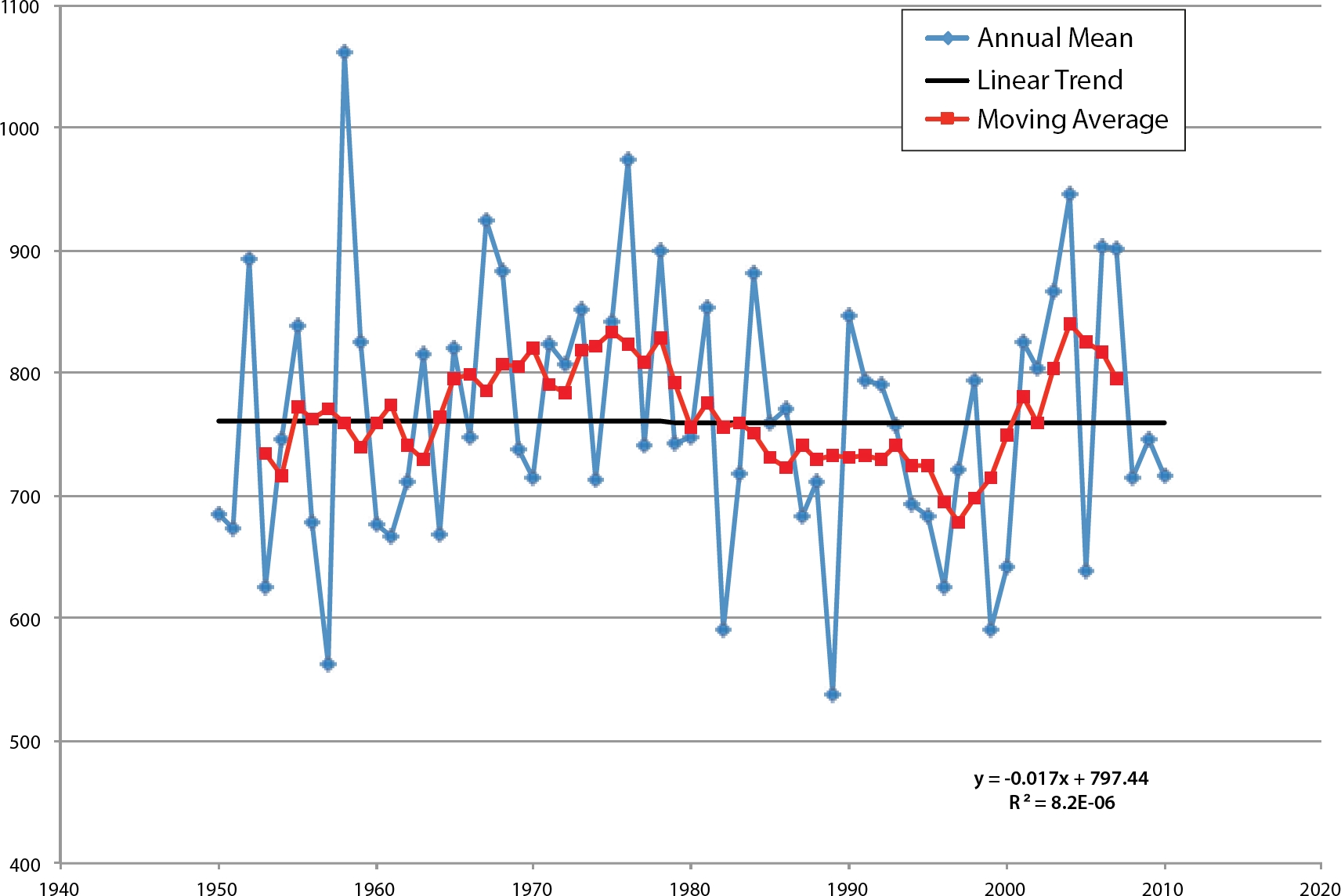
Bravo et al. (2014) confirmed that precipitation in Mexico City shows a similar response to meteorological phenomena affecting it, with a high correlation between seasons. These authors found that the first principal component accounts for 40.5% of the variance and proposed that this first component is the average precipitation. Following their conclusion, the average of all stations included in this study was calculated and analyzed.
Figure 4 shows the linear trend, which demonstrates that during the period analyzed, it does not show a tendency to either increase or decrease; nonetheless, an oscillation occurs involving approximately one full cycle over the period of time studied. This behavior does not show a significant correlation with the Pacific Decadal Oscillation (-0.24) or the Atlantic Multidecadal Oscillation (-0.17), suggesting that it responds in a more complex way to the interaction between them, making it necessary to have a much longer period of data. We can hypothesize that the altitude and continentality of Mexico City are key factors for a reliable study on how climatic variations influence inter-annual variations in this area.
Influence of ENSO on precipitation in Mexico City
ENSO events were classified according to mean annual MEI. As shown in Table 1, seasonal and annual precipitation averages were obtained for each year, and then the spatial distribution during the warm and cold ENSO phases was derived, as well as the neutral phase. The highest precipitation occurs during neutral years, with an average of 1450 mm/year (1200 mm/season for the wet and dry seasons) in the southwest of Mexico City. In addition, during the ENSO warm phase precipitation values range from 550 to 1200 mm/year (1100 and 100 mm/season for the wet and dry seasons, respectively), with a lowest-to-highest trend from the northeast to the southwest. The cold phase shows a similar distribution, with precipitation ranging between 550 and 1200 mm/year (500-1100 and 45-100 mm/season, respectively, for the wet and dry seasons) (Figure 5). The behavior of precipitation in relation to MEI is summarized in Table 2.
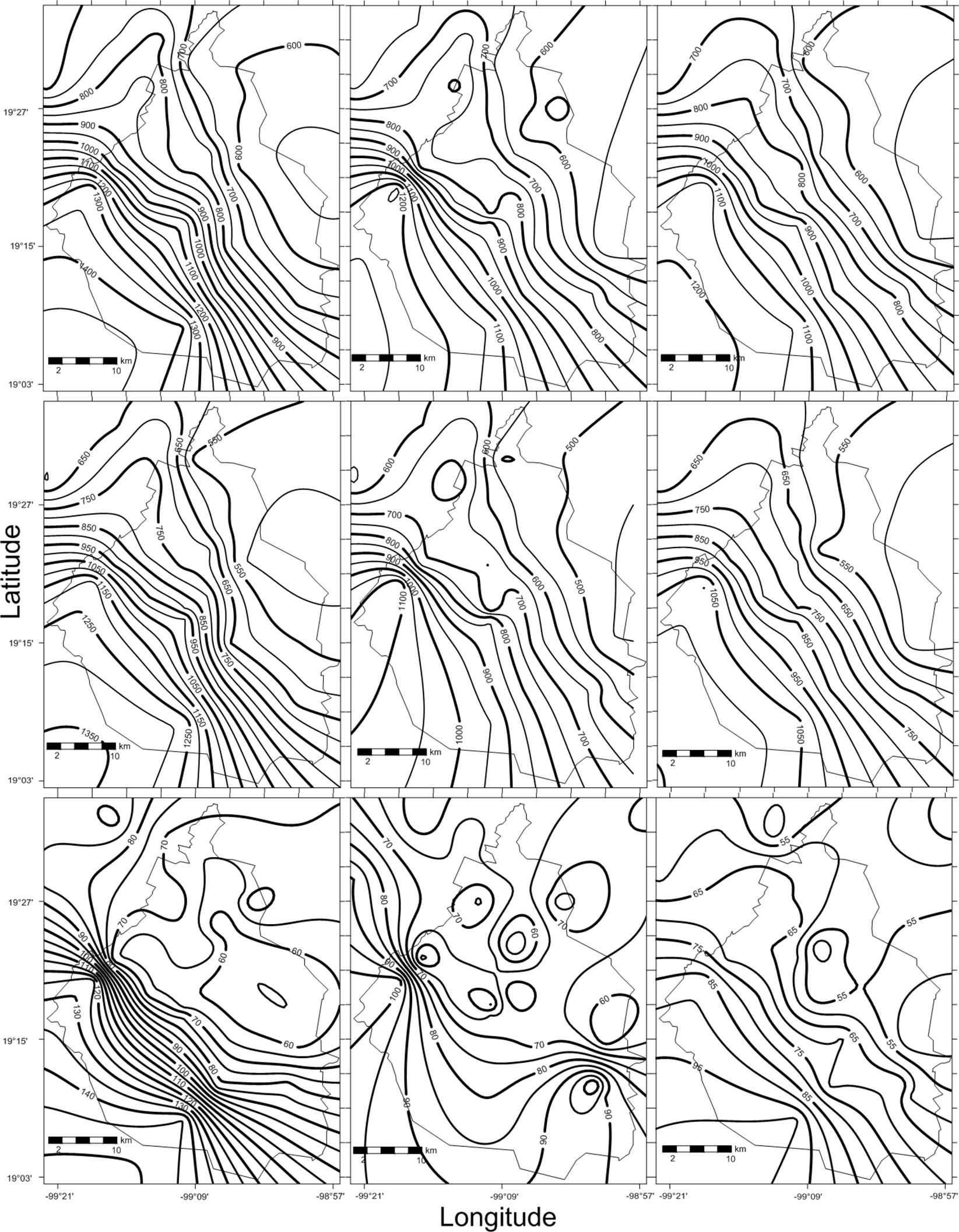
Figure 5 Mean precipitation (mm): rows are annual average (top), May-October (wet season; middle), and November-April (dry season; bottom); columns correspond to neutral years (left), El Niño (center), and La Niña years (right).
Table 2 Precipitation in Mexico City (mm) according to neutral, El Niño or La Niña events for annual wet and dry seasons.
| Neutral | El Niño | La Niña | |
|---|---|---|---|
| Annual | Max=1450<breal></break>Min=550 | Max=1200<breal></break>Min=550 | Max=1200<breal></break>Min=550 |
| Wet Season | Max=1400<breal></break>Min=500 | Max=1100<breal></break>Min=450 | Max=1100<breal></break>Min=500 |
| Dry Season | Max=145<breal></break>Min=50 | Max=100<breal></break>Min=50 | Max=100<breal></break>Min=45 |
Precipitation follows a similar behavior in both the wet and dry seasons,, that is, the highest values occur in the southwest, and decrease towards the northeast. A decrease in rainfall in the southwestern is also observed area during both El Nino and La Nina for the wet and dry seasons (Figure 5).
A different approach is proposed to determine the influence of ENSO on precipitation in Mexico City, by using seasonal and annual averages of the ENSO Multivariate Index, as well as the corresponding rainfall averages for the 31 gauge stations selected. With these values, 3-row × 2-column contingency tables were constructed for which both row and column totals are random variables, i.e., second category of contingency tables (Conover, 1971).
The classification of rows is conducted using mean annual MEI values, according to 3 categories:
El Niño, corresponding to values above 0.5
Neutral, corresponding to values between -0.5 and 0.5
La Niña, corresponding to values below -0.5
The classification of columns was conducted using precipitation values: above or below the median, i.e., the 50th percentile of the sample (747.45 mm/year; 680.18 and 69.68 mm for the wet and dry seasons, respectively). The median was used to avoid biases in the measure of central tendency produced by very high or very low values. The 61-year sample was divided into 2 subsamples: the first between 1961 and 1990, and the second between 1991 and 2008; these years were chosen for including more than 20 stations in the study area. The first period comprises 30 years, which is the number of data needed for calculating climatological normals. This subsampling aimed to derive a hypothesis with one sample and avoid using this same sample to test it, in order not to bias the results.
The annual classification of years is shown in Table 3.
Table 3 Frequencies corresponding to the sub-samples.
| First subsample (1961-1990).<breal></break>Median=747.45 mm/year | |||
|---|---|---|---|
| Above the median | Below the median | Total | |
| El Niño | 2 | 7 | 9 |
| Neutral | 10 | 2 | 12 |
| La Niña | 3 | 6 | 9 |
| Total | 15 | 15 | 30 |
| Second subsample (1991-2008). | |||
| Above the median | Below the median | Total | |
| El Niño | 0 | 7 | 7 |
| Neutral | 5 | 3 | 8 |
| La Niña | 0 | 3 | 3 |
| Total | 5 | 13 | 18 |
The null hypothesis, H0, suggested by the second part of Table 3, is that frequencies are independent of the state of MEI. An independence Chi-square test was performed using the first part of Table 3; however, for this test to be valid, El Niño and La Niña boxes were pooled because of the insufficient number of cases (Conover, 1971; Infante and Zárate, 1984). The resulting table is as follows (Table 4).
Table 4 Complete set of El Niño and La Niña events compared to Neutral events.
| Above the median | Below the median | Total | |
|---|---|---|---|
| Neutral | 10 | 2 | 12 |
| El Niño or La Niña | 5 | 13 | 18 |
| Total | 15 | 15 | 30 |
When performing a Chi-square test with one degree of freedom on the data in this table, the assumption of independence between ENSO and the frequency of precipitation data above or below the median will be rejected with an independent sample from the one that suggested it.
Because the Chi-square test yielded significant differences, it was applied to the entire data set. The result is shown below:
The Chi-square value for this table is 4.91. The rejection region for α = 0.05 is 3.8; that is, the hypothesis of independence between MEI and frequency of years with precipitation above or below the median is rejected. Therefore, the presence of ENSO in its positive or negative phases is related to a reduction in the frequency of years with precipitation above the median, i.e., a decrease in precipitation.
Additionally, following Pavia et al. (2006), the bootstrapping technique (Efron, 1979, Efron and Tibshirani, 1986) was used in order to calculate Table 6 for which uncertainties are known, despite the insufficient number of cases. A total of 150 replicate bootstrapping calculations were performed with the data used for calculating the data shown in Table 5.
Table 5 Frequencies corresponding to the complete sample (1950-2010).
| Median value =747.45 | |||
|---|---|---|---|
| Above the median | Below the median | Total | |
| El Niño | 8 | 10 | 18 |
| Neutral | 18 | 9 | 27 |
| La Niña | 4 | 12 | 16 |
| Niño + Niña | 12 | 22 | 34 |
| Total | 30 | 31 | 61 |
Table 6 Frequencies corresponding to the complete sample calculated by bootstrapping (150 replicate calculations) and their standard deviations. Values in bold confirm the significance (95%) of the values observed (Table 5).
| Above the median | Below the median | Total | |
|---|---|---|---|
| El Niño | 8.8±1.9 | 9.2±1.9 | 18 |
| Neutral | 13.2±2.0 | 13.8±2.0 | 27 |
| La Niña | 8.0±1.7 | 8.0±1.7 | 16 |
| Total | 30 | 31 | 61 |
Bootstrapping shows that the rejection of the independence hypothesis is significant at 95%, and confirms a decrease of cases in which precipitation is above the median in the negative phase (La Niña) and an increase of cases in which precipitation is above the median in the Neutral phase. The probability of occurrence after bootstrapping was calculated from Table 5 and is shown in Table 7.
Table 7 Probability of precipitation occurrence according to ENSO status.
| Complete sample (1950-2010) Median value =747.45 | ||
|---|---|---|
| Above the median | Below the median | |
| El Niño | 44 | 56 |
| Neutral | 67 | 33 |
| La Niña | 25 | 75 |
The same procedure was used for the dry and wet seasons separately; however, Chi-square tests yielded non-significant differences, probably because the low number of useful stations; therefore, only the annual contingency tables were considered valid.
To find a precipitation anomaly during El Niño (La Niña) events, precipitation during neutral years were considered as baseline or reference; afterwards, the difference between this baseline with precipitation during the ENSO phases was obtained, as shown in Figure 6.

Figure 6 Map of annual precipitation anomalies (%) for El Niño (left) and La Niña (right) years, relative to the median of Neutral years.
The eastern region of Mexico City shows a surplus precipitation relative to the median during El Niño events (Figure 6), ranging from 15 to 20 mm (106%), and a deficit of up to 240 mm (82%) in the southwest of the state. For La Niña, the distribution of precipitation is similar: precipitation is higher than the median in the east of the city (40 mm, or 110%), but the areas delimited are larger. Likewise, the difference in precipitation for the rest of the City is similar compared to the map corresponding to the positive phase.
During the positive phase of ENSO, the variation in the position of the Hadley cell contributes to suppressing the ascending vertical air flow that favors precipitation in the southern part of Mexico (Bravo et al, 2017; Magaña, 2004; Douglas et al, 1993; Bhattacharya and Chiang, 2014). Additionally, the activity of tropical cyclones is also suppressed (Jaúregui, 1995).
Douglas et. al (1993) had already noted that precipitation in the northern region of Mexico shows negative rainfall anomalies related to the positive and negative phases of ENSO, arguing that vertical velocity shows negative values in this area. Magaña (2003) and Fuentes-Franco et al. (2018) also report this behavior and argue that the interannual weather variability in this region of Mexico may be related to fluctuations in sea temperature over the eastern Pacific Ocean. The results of this work confirm that the area of negative precipitation anomalies reaches the center of the country. The explanation partially lies in the fact that the strongest trade winds and tropical disturbances cause the associated humidity to be transferred to the southern region, causing a decrease in rainfall in the northern and central parts (Mosiño and Morales, 1988).
CONCLUSIONS
Precipitation in Mexico City shows a clear lower-to-higher trend in from the northeast to the southwest, and despite the low number of stations in the latter, the results confirm previous findings; however, these results should be interpreted with caution.
The relationship of Mexico City precipitation and ENSO is complex; nonetheless, this analysis suggests that negative ENSO phases lead to lower precipitation levels in Mexico City, as the probability of above-median rainfall decreases; the neutral phase is associated to higher precipitation and a lower probability of below-median rainfall. During the positive phase, precipitation is not significantly affected.
Under neutral ENSO conditions, rainfall ranges from 550 mm/year in the northeast to 1400 mm/year in the southwest; during the positive or negative phases, precipitation decreases mainly in the southwestern area, with a deficit reaching 150 and 200 mm/year, respectively.
During the period 1950-2010, mean annual precipitation does not show a significant trend to either increase or decrease. It shows a virtually complete cycle over the study period. As longer time series become available, these will support a more in-depth analysis of this behavior.
These results contribute to predict precipitation in Mexico City, as higher or lower precipitation levels may be expected according to the El Niño forecast.

