Introduction

Performing risk quantification analyses for portfolios conformed of crude oil and refined products is an important issue for refiners, integrated oil companies and any other entity that is particularly exposed to portfolios with short and long positions on these products. Clearly, one of the most important risk factors affecting financial results and determining the cash flows at risk in this type of entities is the spread between the prices of these energy commodities.

The differential between these prices is commonly known as refining margin, and it is a key factor in determining profits and losses of the aforementioned entities to a greater or lesser extent. As mentioned in ^{García Mirantes et al. (2012)}, “Refining is a margin business,” so refiners’ profits, in particular, are essentially independent of oil and product prices in nominal terms. In other words, the profits of a refining company depend only upon the difference between the prices of crude oil and the refined products. Integrated oil companies, on the other hand, are exposed to both: crude oil and refined product price levels and the refining margin itself to varying degrees.

It can be inferred that having models that make it possible to adequately replicate the behavior of the refining margin is fundamental for the valuation of portfolios composed of crude oil and its refined products, and their appropriate implementation constitutes a major challenge for companies in the oil industry. With this type of models, integrated oil companies and refineries can generate different scenarios that they might face during a project or fiscal year and thereby assess potential economic performance to consider in the decision-making process.

When it comes to the behavior of the refining margin, it is important to bear in mind that, as pointed out in ^{García Mirantes et al. (2012)}, the spread between these commodity prices does not always rise when both the crude oil price and that of the corresponding commodity increase, and contrariwise. Therefore, analysts must be cautious when selecting a model should they be willing to replicate this feature of the spread behavior.

Several studies have aimed at finding the main factors determining the spread distribution between crude oil and its refined product prices. For instance, the results of econometric analyses carried out by ^{Kauffmann and Laskowski (2005)} claim to show that the behavior of the spread between motor gasoline and crude oil prices can be attributed to refinery utilization rates and inventory behavior, whereas contractual arrangements between retailers and consumers is argued to be one of the main factors that explain the behavior of the spread between home heating oil and crude oil prices.

As summarized in ^{Zhang et al. (2015)}, among other factors that have been argued to explain the behavior of the spreads between crude oil and refined petroleum product prices over time are: physical storage availability, transportation constraints, the driving season, and technological changes on the demand side.

The spread-driving factors mentioned above are usually variables whose value is not feasible to model when attempting to carry out simulation analyses for risk quantification purposes. Additionally, they may become less relevant when carrying out long run risk management analyses. Given this, the aforementioned factors will not be explicitly incorporated into the spread modeling process in this study.

There has also been an intensive discussion around whether the relationship between the prices of crude oil and refined petroleum products is asymmetric when analyzing co-movements of these prices. Numerous studies that explore the relationship between crude oil and refined petroleum product prices, such as ^{Kaufmann and Laskowski (2005)}, claim there is an asymmetric response of refined petroleum product prices -gasoline in particular- to crude oil price movements, whereas in recent analyses, ^{Zhang et al. (2015)} argue that a threshold error correction model reveals an “almost symmetric” relationship between the prices of these commodities.

For the purposes of this paper, whether or not an asymmetric relationship exists between the prices of crude oil and refined petroleum products shall not be taken into consideration, since as we will explain later, the value of the spread between crude oil and refined petroleum products will be modeled without explicitly considering variable co-movements. Additionally, and also to be explained later, evidence has not been found in this study of co-movements between the crude oil price and the spread between this commodity and the crude oil and refined petroleum products price differentials.

Unfortunately, it is not common in the literature to find models that adequately emulate the behavior of the aforementioned price differentials, previously referred to as refining margins, and are, therefore, suitable for performing risk quantification analyses. In contrast, research regarding price differentials usually focuses on the development of models generally designed and calibrated to estimate the price of energy spread derivatives, such as options, forwards and swaps, as their main objective, but we barely find models aimed merely at carrying out risk quantification analyses.

Thus, since valuation of derivatives is the main objective for developing the most popular price differential models, they are designed under the risk neutral probability measure and may, consequently, be inadequate for risk quantification analysis.

Carmona and Durrelman (1998), for instance, focus their study on demonstrating how Kirk’s formula provides an accurate approximation for pricing options but do not spend time proving whether the mathematical framework used to model price differentials is appropriate to describe the behavior of the spreads whose options are to be priced. This kind of model allows the spreads to take on unrealistic values in the long run. Most of the existing models may not, therefore, be the most appropriate for using as risk management tools.

When modeling stochastic variables, it is important to keep in mind that if aiming to carry out risk quantification analyses, the main objective in selecting an appropriate model must be to avoid choosing one that either overestimates or underestimates the actual risk embedded in the variables to be analyzed. Ideally, a model should be selected that does not only avoid these mismeasurements but also best describes the behavior or the risk factors.

Consequently, the hypothesis for this research consists of checking whether the development of a model based on first-order Markov chains, under the real probability measure, could be considered a more efficient tool for carrying out risk measuring necessary for company decision-making. To this end, the performance of such a model should be compared with the results offered by some of the most popular models for price differentials in the known literature.

In addition, this model can be used to evaluate projects such as the revamping and rehabilitation of a refinery or a refining system, like future ones planned for Mexico, in order to identify if such projects might be profitable, as well as the probability of them being more profitable than required by such projects.

Thus, the two main contributions of this research are: i) to provide a model for energy product price differentials based on first-order Markov chains, and ii) that the model will be based on dynamic transition matrices and conditioned to the price range containing crude oil, as an explanatory variable.

Section I will provide a literature review of some of the most popular existing one-factor models for energy spreads. Section II will present the definition of the variables we will be working with, their main features and the model fitting issues found through exploratory data analyses, as well as an explanation of some of the main limitations of the existing one-factor models presented in section I as risk management tools. Section III will introduce our proposed model for energy spreads, based on empirical distribution and using switching first-order Markov chain Monte Carlo simulation. Finally, section IV will compare the results of a risk quantification analysis carried out with two different models, the first one using the correlated two-factor Clewlow and Strickland model to simulate the individual legs of the spread between crude oil and gasoline prices as correlated variables, and the second obtained from the model proposed in section III and showing how it can help avoid misquantifications in this kind of analyses.

I. The current framework: most popular one-factor models

For spread modeling, ^{Blanco et al. (2012)} introduce some of the most popular methodologies to model two-asset price spreads and explain their main uses and limitations. While presenting these models, the authors emphasize one critical question that any analyst must deal with before modeling spreads. This question is “whether to model the spread explicitly as a stochastic variable or to model the individual legs of the spread as correlated variables.”

In this section, some of the most popular methodologies for modeling two-asset price spreads will be introduced. Later, section II will present the price differentials we will be working with and analyze their behavior to determine whether these models are appropriate for the energy spreads involved.

As mentioned in ^{Blanco et al. (2012)}, one of the first models proposed for the spread between two asset prices is based on the assumption that this risk factor could follow a lognormal distribution and that it could be estimated through a one-factor model, as the one used in the well-known Black model.

As explained in the study mentioned above, the main reason for researchers making this assumption is that since the primary purpose of using this model is to be able to value spread options by standard option pricing tools, it should be estimated under a risk-neutral measure. One of the main weaknesses of the model is that it does not allow for negative values. The next section will verify whether this results in an adequate assumption for the energy spreads being studied.

Now on to the second most popular one-factor model, presented by ^{Poitras (1997)}, the Wilcox Spread Option Formula, carried out for cases where prices would follow an arithmetic Brownian motion. With this model, changes in the spread are assumed to be normally distributed variables. This assumption does allow negative values for the spread, so the problem identified with the first model seems to be taken care of. The arithmetic Brownian spread process is given by:

As an improvement, a mean-reversion factor with a mean-reverting fixed level can be incorporated to this normally distributed one-factor model. The stochastic spread process equation appears below:

This process corresponds to the continuous time analogue of the discrete time AR(1) process and is pulled towards an equilibrium level S- at a rate α with volatility σ per square root time. To determine the stochastic integral of this process, a variation of parameters procedure is required. To do this, it is necessary to define a new function:

Finding the derivative via Ito’s lemma, we obtain

Integration from t to T gives

where ε~N(0,1). At this point, it is important to highlight that the main handicap of this model is that it results in a symmetric distribution.

So far, we have reviewed the most widely used one-factor models. In the next section, we will introduce the energy price differentials subject to the investigation and analyze the main features of those energy spreads, to verify whether the models presented above could be suitable for any of them.

II. Variables: definition, main features and model fitting issue

Although, as we will see later, without assuming the spread between refined petroleum products and the level of crude oil prices to be totally independent, in this section we aim to show why the spread should be modeled as an explicit stochastic variable, consistent with the one-factor models presented in ^{Blanco et al. (2012)}.

To prove this statement, we worked with prices of the NYMEX Division New York Harbor unleaded gasoline blendstock for oxygen blending (RBOB), New York Harbor ULSD heating oil (Diesel) and West Texas Intermediate crude oil (WTI) first month future contracts. Historical data from November 2003 to April 2017 were used to carry out the analysis presented below (source: Bloomberg; first month future contracts).

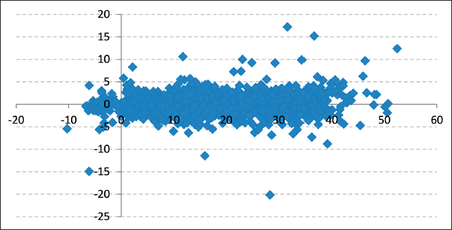
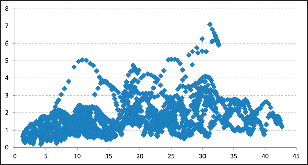
Firstly, the spreads between RBOB and WTI (RBOB-WTI Spread) and Diesel and WTI (Diesel-WTI Spread) prices were obtained in U.S. dollars per barrel. Secondly, the day-to-day changes in these two spreads as well as the changes in WTI prices in absolute terms were calculated. Thirdly, both, the correlations for the full period and those based on one year rolling window for the changes in RBOB-WTI Spread and WTI price levels and for the changes in Diesel-WTI Spread and WTI prices were calculated. Scatter plots, as well as rolling window correlation graphs, are shown below.

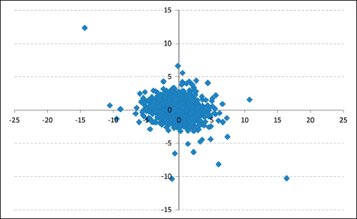
As the scatter plots (Figures 2 and 4) show, neither changes in the RBOB-WTI Spread nor changes in the Diesel-WTI Spread seem to show any correlation with changes in WTI price levels. In addition, the rolling window linear correlation graphs (Figures 1 and 3) show that linear correlations are far from stable given that they move from positive to negative values throughout the period of study. Based on this, it would be natural to infer that there is no empirical evidence to assume the existence of either a positive or negative linear correlation between the two series.

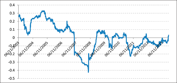
Figure 1 One-Year Rolling Window Correlation between Changes in RBOB-WTI Spread and WTI Price Changes. 

Figure 2 Scatter Plot of Changes in RBOB-WTI Spread vs. WTI Price Changes. 

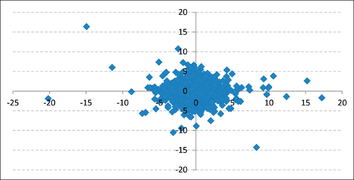
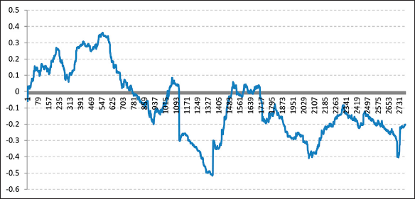
Figure 3 One-Year Rolling Window Correlation between Changes of Diesel-WTI Spread and WTI Price Changes. 

Figure 4 Scatter Plot of Changes in Diesel-WTI Spread vs. WTI Price Changes. 

Nevertheless, statistical tests were run to verify the findings. The cross-correlation function was obtained to corroborate whether there is a linear correlation between changes in both spreads and crude oil price changes, and findings show that in both spread cases, the correlation exceeds the 95% confidence interval for some function lags.

Figure 5 Cross Correlation ∆wit vs. ∆(WTI-RBOB). 

Figure 6 Cross Correlation ∆wit vs. ∆(WTI-Diesel). 

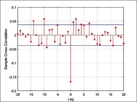
Notwithstanding, given that all values in the cross-correlation function were low (less than 0.17), additional tests were carried out by sampling several different sizes in the data.

The sampling showed no consistency in lags of the correlation function for which confidence levels were exceeded, so no significant correlation can be concluded for any particular lag. Moreover, the cross-correlation level changed from positive to negative depending on the sample.

Finally, to complement the linear correlation verification, a zero cross-correlations test was performed on the full data and various samples resulting from sampling. Known as the “multivariate portmanteau,” the test consists of proving the null hypothesis H0:ρij=0∀i,j=0,1,…m versus the alternative hypothesis Ha:ρij≠0 for some i, j. The tests reveal that the correlations for some samples can be considered statistically equal to zero, whereas there is rejection of white noise for some others. Since no consistency was found by carrying out this test, cross-correlation between price differential changes and crude oil price changes can be rejected in both cases (RBOB-WTI and Diesel-WTI Spreads).

As a result of this, it can be concluded that modeling the RBOB-WTI Spread and the Diesel-WTI Spread as explicit stochastic variables without incorporating co-movements between them and WTI crude oil price results appropriate for these price differentials. The next section of the paper will quickly review some of the most popular models proposed for these price spreads and discuss their potential effectiveness as risk management tools.

II.1. Assessing the Lognormal Model

Considering that with the lognormal model, energy spreads would follow the process shown in equation (i), it can easily be observed that this would result in an unrealistic assumption for most of the energy price spreads. It is particularly inadequate for the crude oil and RBOB gasoline spread, since as seen in the graph shown below (see Figure 7), the RBOB-WTI Spread can take on negative values even if only for short periods of time, while that could never happen with a lognormal distribution for spreads.

Figure 7 Historical Behavior RBOB-WTI Spread. 

Figure 8 Historical Behavior Diesel-WTI Spread. 

In the case of Diesel-WTI Spread, there is not enough empirical evidence to up-hold that the price differential can have negative values, although values below zero should not be discarded given the nature of the variable. In any event, to verify whether the Diesel-WTI Spread could be considered to follow lognormal distribution, the assumption of ln (Diesel-WTI Spread) following a random walk was tested.

The Homoscedastic Increments test was used for this. In other words, we tested whether there is statistical evidence that variance of ln(S_t ) - ln (S_t-2 ) could be considered to be twice the variance of ln(S _t ) - ln (S_t-1 ) and whether the variance of ln( S_t ) - ln (S_{t -3}) could be considered to triple the variance of ln(S_t ) - ln (S_t-1 ). From this point forth, we shall denote S_t as the value of the spread we are studying at time t.

The results of the test show that the assumption that ln(Diesel-WTI Spread) follows a Random Walk must be rejected (statistics are shown in Table 1); the errors of the variable ln(Diesel-WTI Spread) do not behave as independent and identically distributed Gaussian random variables. Consequently, the lognormal model is not an appropriate model for this price differential.

Table 1 Homoscedastic Increments Test for ln(Diesel-WTI Spread). 

μ σa2 σb2	0.00060 0.00715 0.00635
(2n)0.5Jd z0.05σa2*(2*2)0.5 z0.95σa2*(2*2)0.5	-0.06088 -0.01663 0.01663
(2n)0.5Jr z0.05*20.5 z0.95*20.5 z0.025*20.5 z0.975*20.5	-8.51815 -2.32617 2.32617 -2.77181 2.77181

With 95% confidence, the hypothesis of errors being independent and identically distributed is rejected.

As additional evidence to test lognormal distribution assumption, the implication that “the spread volatility in absolute terms would increase as the size of the spread increased” was verified, in line with what ^{Blanco stated (2012)}. Even though we have already provided evidence that the lognormal assumption for RBOB-WTI and Diesel-WTI Spreads does not result in an adequate assumption, these final tests were performed to verify for both spreads whether volatility increases in absolute terms as size augments.

First, using a one-month rolling window and the one-month spread level average, the standard deviation of the spreads was calculated for each of the two spreads. Additionally, the scatter plot for the levels of the spreads versus the value of their absolute changes was obtained. The resulting graphs are shown below (see Figures 9 to 12).

Figure 9 RBOB-WTI Spread Level vs. RBOB-WTI Spread Changes. 

Figure 10 One-Month Moving Average vs. One-Month Rolling Window Volatility of RBOB-WTI Spread. 

Figure 11 Diesel-WTI Spread Level vs. Diesel-WTI Spread Changes. 

Figure 12 One-Month Moving Average vs. One-Month Rolling Window Volatility of Diesel-WTI Spread. 

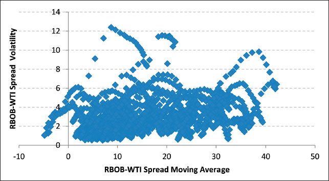
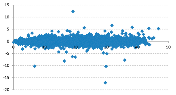
As seen in the scatter plots of both the RBOB-WTI and Diesel-WTI spread levels versus changes, there is no evidence that high spread levels imply greater changes in the spreads. Also, comparing one-month rolling window volatility with their respective one-month moving average graphs does not show any clear relationship between RBOB-WTI and Diesel-WTI spread levels and their respective volatility.

Finally, an F-test to prove equal variance was carried out for different levels of the spreads. Although findings showed that for some levels of the spreads the null hypothesis of equal variance should be rejected, for some cases in the medium and high spread levels the assumption of equal variances holds with 95% confidence for both spreads.

It can thus be concluded that assuming lognormality to model RBOB-WTI and Diesel-WTI spreads is inadequate considering the behavior of crude oil and refined petroleum product spreads.

III. Model: an alternative methodology to simulate the value of price spreads

So far, we have observed that some of the most popular methodologies for modeling the value of spreads between crude oil and refined petroleum products -as explicit stochastic variables- contain important model risks for carrying out risk quantification analyses. In this section, an alternative methodology for modeling the value of this type of spreads will be introduced. In the scope of this study, we will particularly focus on modeling the value of the RBOB-WTI Spread.

It is important to bear in mind that the main purpose of the methodology proposed here is to provide analysts with a risk management tool for risk quantification and not for valuation of spread derivatives, as opposed to ^{Poitras (1997)} and ^{Blanco et al. (2012)}, whose main goal is to price these hedging instruments and for which some of the main handicaps are inconsistency with the absence-of-arbitrage accomplishment and lack of market pricing information. In other words, the methodology proposed herein is intended be used for quantification of risk in the real world in contrast with that used in most models, which is designed to carry out risk-neutral pricing. Since the models designed to price derivatives incorporate market expectations about future spread value for both the risk-neutral expected value (based on either the forward or future values of the spread) and implied spread volatility (usually obtained from option prices), using the methodology we propose would lead to significantly different values from those quoted in the market, given that these values neither can be nor are intended to be integrated in the model.

The proposed methodology consists of a simple model based on switching Markov chain Monte Carlo simulations, where the Markov chain determining the spread level changes will depend on the crude oil price level. Thus, the value of the Crude Oil and Refined Petroleum Product Spread at time t will not only depend on the value of the spread at time t-1 but also on a simulated value of the crude oil price at time t. The latter price will be simulated by one of the most popular models for commodity prices, which will be introduced later on: the Clewlow and Strickland model.

The motivation for proposing a spread level model that depends on both the value of the spread at time t-1 and the value of crude oil price at time t is that after carrying out exploratory data analysis, it was found that the values that RBOB-WTI Spread have taken over time do vary depending on variations in crude oil prices. To show this, we will first present the scatter plot of the values of the RBOB-WTI Spread versus the WTI crude oil price levels (see Figure 13).

Figure 13 RBOB-WTI Spread vs. WTI Crude Oil Price. 

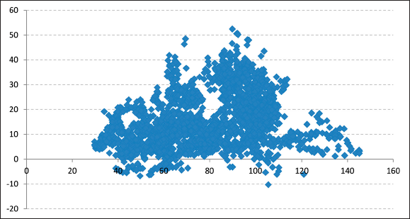
As seen in the chart, when crude oil values have fallen below levels of around U.S. 60 dollars per barrel, the price differential between crude oil and RBOB gasoline has not exceeded levels of U.S. 30 dollars per barrel.

In order to test whether this empirical result is statistically significant, in other words whether significant differences exist between the behavior of the RBOB-WTI Spread when the WTI crude oil price has fallen below U.S. 60 dollars per barrel and the behavior when this crude oil price has been above that level, the following steps were carried out.

First, the RBOB-WTI Spread sample was divided into six subsamples of approximately equal size stratifying the sample based on the prices of the RBOB-WTI Spread crude oil price from lowest to highest, two of them corresponding to values where the WTI crude oil price has fallen below U.S. 60 dollars per barrel and four of them to values above this price.

Secondly, the hypothesis of same means and same variance under normal distribution assumption was tested for each pair of samples.

Finally, the two-sample Kolmogorov-Smirnov test was used to test equality of these continuous one-dimensional probability distributions.

As a result, statistical evidence was not found to reject the hypothesis that sample 1 and 2 below are equally distributed. In other words, the same mean and same variance hypothesis was accepted with 99% confidence. Moreover, based on the Kolmogorov-Smirnov test we can consider that samples 1 and 2 follow the same distribution.

Similarly, for samples 3, 4, 5 and 6, the samples corresponding to the range where the WTI crude oil price has taken values above U.S. 60 dollars per barrel, it was found that the null hypothesis of same mean and same variance was accepted with 99% confidence. Regarding the Kolmogorov-Smirnov test, even though the null hypothesis of equal distribution was rejected for some pairs of samples, the hypothesis of the RBOB-WTI Spread crude oil having the same distribution throughout the range can be considered to hold where the WTI crude oil price has taken values above U.S. 60 dollars per barrel.

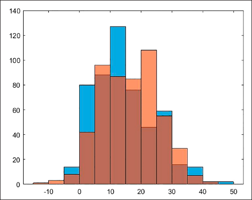
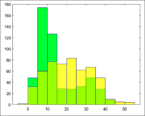
On the other hand, the null hypothesis of distribution of samples 1 and 2 having same mean, same variance and following the same distribution as samples 3 to 6 has been rejected in all cases. Based on this, we can assume there is sufficient empirical evidence to determine the null hypothesis that the RBOB-WTI Spread crude oil has the same distribution for the range where the WTI crude oil price has taken values below U.S. 60 dollars, and the range where WTI has been above this value must be rejected. The plots of some pairs of distributions are shown below (see Figures 14 to 17) only for illustrative purposes.

Figure 14 Histogram Sample 1 vs. Sample 2. 

Figure 15 Histogram Sample 2 vs. Sample 3. 

Figure 16 Histogram Sample 1 vs. Sample 2. 

Figure 17 Histogram Sample 2 vs. Sample 3. 

Nonetheless, as will be explained later, our simulation model will allow for the existence of RBOB-WTI Spread values above U.S. 30 dollars per barrel for WTI crude oil price levels, although with a lower occurrence probability than that estimated for different crude oil price ranges.

The classification described above is based on empirical data, and the determination on how the crude oil price ranges must be partitioned will vary depending on the behavior of the crude oil and refined product spread to be analyzed. Quantitative risk management analysts must perform a similar type of statistical analysis when working with the price spread between crude oil and other refined petroleum products. The goal here is to be able to identify the crude oil price levels where spread behavior presents different distribution, in order to be able to carry out the steps of the procedure that will be described below.

Hence, we will initially work with two transition probability matrices corresponding to each of the aforementioned WTI crude oil price ranges. As commonly done, the values of the RBOB-WTI Spread must be discretized to use the first-order discrete-time Markov chain methodology. In this particular case of study, the values of the spread were divided into 21 equally spaced ranges, and one probability transition matrix was obtained for each of the two different WTI crude oil price ranges, as described above.

At this stage, it is important to recall that the first-order discrete-time Markov chain with m states satisfies the following relationship:

with m possible states for each value k_t. Thus, the form of the original probability transition matrices is as follows:

for i equals to 1 or 2, according to each one of the ranges of prices of WTI crude oil described above. Thus, M⁽¹⁾ is the matrix resulting from the RBOB-WTI Spread behavior observed when the crude oil price is below U.S. 60 dollars per barrel; and M⁽²⁾ is the one resulting from the RBOB-WTI Spread behavior observed when the crude oil price is above U.S. 60 per barrel.

These two probability matrices will be the starting point for modeling the RBOB-WTI Spread value. As we will see shortly, these matrices will only be the input for the final probability matrices driving the movements on the RBOB-WTI Spread.

The methodology proposed here aims to enable switching the Markov chain driving the RBOB-WTI Spread movement, S_t , based on the simulated price of WTI crude oil at time t, denoted as X_t from here on. Thus, the probability matrix driving the movements of the RBOB-WTI Spread from state to state will depend on an additional parameter, θ, that will be a function of the value of the WTI crude oil price at time t. To this end, in the model proposed herein, the value of the RBOB-WTI Spread in each simulation will be obtained through the following equation:

where St* is the value of the simulation of the RBOB-WTI Spread obtained from Markov chain Monte Carlo simulations, coming from what shall be called the Ruling Matrix at time t, M_t , which is, in turn, a function of θ(X_t) and M_t-1 ; ω_t´s are independent random variables uniformly distributed [0,1]; and a is the length of the equally spaced RBOB-WTI Spread ranges.

The main objective of including parameter a and the random variables ω_t is to be able to obtain values for the RBOB-WTI Spread all along each range where the spread has taken values. A slight variation for this random variable corresponding to the states at the tails of the spread distribution can be proposed; however that would require further analysis to determine an adequate distribution for the tails. For the purposes of this study, extreme value analysis was not carried out to describe the potential behavior of the tails. In further analysis, a proposal for this distribution will be presented.

Thus, the form of the Markov chain probability matrix driving the value of the discrete value of the RBOB-WTI Spread at time t, St*, is a function of the Ruling Matrix, M_t , defined above, given the value of St-1*, as is common practice.

We will then describe the way in which the Ruling Matrix, M_t , will be constructed based on matrices M ⁽¹⁾ and M⁽²⁾, the smoothing parameter θ(X_t) and the value of the Ruling Matrix at time t - 1, M_t-1 , at a particular point in time. We must first point out that the value of M_t will be different for each simulation, since it will be path dependent and it is a function of the value the crude oil, X_t , takes at any particular time. The adjustments performed to get to on each path lead us to probability matrices as described below.

Now, as can be inferred, the initial value of the Ruling Matrix M₀ will depend on the value the WTI crude oil price takes at time zero, X₀, that is, if the value of X₀ is below U.S. 60 dollars per barrel then M₀ = M⁽¹⁾; otherwise, M₀ = M⁽²⁾. Hence, we now have the value of M₀, based on which the following values of M_t will depend.

To describe the next step in the methodology to build M_t , it is relevant to notice that the range of crude oil values where more observations were obtained is the higher range, where the WTI crude oil price has taken values above U.S. 60 dollars per barrel.

Based on the data we selected to work with, we observe that throughout our sample, the proportion of times WTI crude oil has fallen below U.S. 60 dollars per barrel corresponds to around 61% of the proportion of times it has risen above it. Based on this, when X_t < U.S. 60 dollars per barrel we will have that θ(X_t ) = 61%/161%; conversely, when X_t ≥ U.S. 60 dollars per barrel θ(X_t ) = 100%/161%. Thereon, the probability Ruling Matrix driving the value of the RBOB-WTI Spread will be set up as:

where I(X_t < 60) = 1, when X_t < U.S. 60 dollars per barrel, and I(X_t < 60) = 0, otherwise.

It is important to bear in mind that there can be as many matrices M⁽ⁱ⁾ as different distributions are observed in the exploratory data analysis described at the beginning of this section and therefore as many values of M⁽ⁱ⁾ as the number of distributions found.

We have now presented a model to simulate the value of the RBOB-WTI Spread that agrees with the historical behavior of this differential of prices through first-order Markov chains. As an additional feature for the model, we integrated the dependence of this spread behavior with the different WTI crude oil price levels. In our next section, we will introduce one of the most popular one-factor models to simulate commodity prices. This model was used to simulate both the WTI crude oil price used to run the spread modeling methodology presented in this section, and the RBOB gasoline value, in order to compare a two-factor model simulation of the spread with the model proposed here. The results of carrying out risk quantification analysis with both models are shown and compared in section 4.

IV. Empirical estimation: model comparison for risk quantification analysis

So far, we have introduced a model to simulate the value of the RBOB-WTI Spread based on a switching Markov chain. As we have seen in the previous section, the feasible values that the RBOB-WTI Spread can take can be assumed to depend on the observed value of the WTI crude oil price and were modeled accordingly.

In this sense, a model for simulating the prices of WTI crude oil must be selected. For this section, we have chosen to model the future prices of WTI crude oil through one of the most popular models used by practitioners, the One Factor Model proposed by ^{Clewlow and Strickland (1999)}.

As proposed in the Clewlow and Strickland article, this model is adjusted by using the stochastic evolution of the energy forward curve of the WTI crude oil. The model is based on the assumption that the forward price curve, F(t, T), has a negative exponential form and thus follows the stochastic differential equation shown below.

As can be observed, the model has two parameters for volatility: parameter σ determines the level of spot and forward price return volatility, while α determines the declining rate for the increments of volatility in maturity forward prices and is also the speed of mean reversion of the spot price. The importance of parameter α is that it also represents the speed of mean reversion of the spot price, which is the variable we will be simulating for the purposes of this paper.

As explained in their article, Clewlow and Strickland’s model for the forward price curve implies that the spot price process follows the stochastic differential equation shown below:

The equation (xii) is consistent with the initial forward curve F(0, T); in other words, through this equation the expected value of X_t at time s is F(s, t)_, maintaining the behavior of the forward curve rate, and makes the long term risk adjusted drift, µ(t), a function of time as follows:

From the equation shown above, it can easily be shown that lnX_T is normally distributed with the parameters specified below:

In order to calibrate the one-factor model presented above based on forward curve prices, the following methodology can be implemented.

Finally, parameters α and σ can be obtained by adjusting a linear regression of the logarithm of the equation shown below using the different volatility maturities found in step (ii).

The value of t for the equation (xv) is zero at all times, since the data we count on correspond to the value of the future prices that we can obtain is equal to F(0, T) for the different maturities selected.

At this point, it is important to highlight that after finding the value of the parameters α and σ the expected value of the spot price process does not necessarily need to be centered at the future price curve current level, which means it no longer has to agree with the risk-neutral prices usually used for valuating commodity derivatives.

The reason for this is simple. Given that we are aiming to carry out risk quantification analyses, the expected values employed must be those that the analyst considers most adequate for risk management purposes. Thus, the equation for the adjusted drift, µ(t), can be rewritten as:

where X-t is the expected value at time t of the commodity that the risk analyst estimates as the most adequate to perform risk quantification analyses. Thus, X-T denotes the curve of expected values estimated by the analyst for the different maturities to be considered in the analysis.

The one-factor model presented above can clearly be used to simulate the prices of more than one commodity at a time by incorporating the correlation of the commodities to be analyzed. This is done by calculating the variance-covariance matrix of the commodities while simulating commodity prices. The variance parameter employed in this variance-covariance matrix is the one obtained during the calibration of the model, while the correlation parameter is estimated from the logarithmic changes of the prices of the commodities to be analyzed.

It is important to introduce this methodology for modeling the future prices of a commodities portfolio, since the results coming from the model proposed in our previous section will be compared with those obtained from the two-factor model simulation of the spread obtained from modeling the prices of WTI crude oil and RBOB gasoline through this methodology.

For the example of risk quantification we will present in this section, we will assume a company is managing a portfolio conformed of a short position of crude oil of 10,000 barrels per day and a long position of RBOB gasoline of exactly the same amount.

This is by far an unrealistic assumption, since as we know, crude oil can be broken down in refineries into several components among which, aside from gasoline, diesel, jet fuel and fuel oil can be obtained. We decided, however, to keep it simple for the purpose of the analysis.

First, the model for simulating the value of the crude oil price for a period of one year was calibrated using the methodology presented above. The values of parameters α and σ obtained were 0.37 and 28%, respectively, while those of α and σ for the RBOB gasoline used in the two-factor model were 0.8 and 31%, respectively.

For this particular analysis, the value of crude oil and the RBOB gasoline for the year of analysis were centered on the future curves, in order to be able to compare the results of the proposed model with the two-factor model using the usual calibration. The values considered for these scenarios are shown in the graph below (Figure 18).

Figure 18 WTI and RBOB Future Prices. 

By using this scenario and the model proposed in the previous section based on the switching Markov chains, the value of the RBOB-WTI Spread and therefore the value of RBOB gasoline were obtained for each simulation of the WTI crude oil price. The same values were obtained with the two-factor model resulting from simulating the prices of WTI crude oil and RBOB gasoline through the methodology explained above. The results of the risk quantification analysis are described below.

Cash flow distributions corresponding to one year of operations with each of the two methodologies are shown in the following graph (Figure 19).

Figure 19 Probability Distribution. 

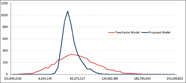
The two-factor model overestimates company cash-flow volatility compared with the one given by the Markov chain model. The volatility of the two- factor model (in dollars per barrel) is equal to U.S. 10.40 whereas the volatility of the Markov chain model equals U.S. 3.90.

Assuming that net operating costs, the minimum value that the proposed portfolio could take for the company not to have losses, was U.S. 35 million (the breakeven value), we calculated the probability of company net cash flow being below this value. Whereas calculated with the two-factor model, the probability of having losses is 25%, with the proposed model it is barely 0.7%. From these figures we can easily see this probability is highly overestimated.

Also, with both methodologies, we calculated cash flows at risk with 90% and 95% significance levels. The two-factor model estimation of this value is of U.S. 20.2 and U.S. 32.5 million dollars respectively, while the proposed methodology yields values of U.S. 0.38 and U.S. 3.09 million dollars.

Finally, the expected shortfall with 95% confidence for the two-factor model equals U.S. 45.4 million dollars, whereas the proposed method produced an expected shortfall of U.S. 6.4 million dollars.

Conclusions

The model proposed here outperforms existing one-factor models, since it enables the existence of negative price differential values and makes it possible to maintain the asymmetry observed empirically by these price spreads, avoiding misquantification of risk.

Also, it was shown that the assumption of equal distributions for the price differential in two different ranges of the WTI crude oil price was not rejected, based on the results of the Kolmogorov-Smirnov tests. From these results, it was concluded that it was appropriate to model the RBOB-WTI Spread price differential based on the values that the WTI crude would take.

On the other hand, while comparing the results obtained by the proposed model and the Clewlow and Strickland two-factor model (CSM), it was found that significantly higher volatility was generated by the CSM than by the one Transition Matrix Model.

In addition, the risk metrics presented above demonstrate that the two-factor model, which is one of the most commonly used to simulate the value of spreads, tends to overestimate the risk embedded in cash flows. This is a common characteristic of most models aimed at derivative pricing and not risk quantification. This overestimation can be misleading when wanting to make decisions based on the risk quantification analysis. While we are well aware that fine-tuning the proposed model to deal with the tails of the empirical distribution would be desirable, the model presented here is considered more appropriate to be used as a risk management tool for decision-making by companies in the oil industry, either for investment in new projects or for the evaluation of their potential results.