text new page (beta)
 English (pdf)
 Article in xml format
 Article references
 Send this article by e-mail
 Cited by SciELO
  Similars in
SciELO
Similars in
SciELO 
 Permalink
1. Introduction
Fogs are phenomena characterized by horizontal visibility reduced to 1000 m or less (WMO, 2017). They can cause significant impacts on various human activities. The transport sector, for instance, is extremely affected by the occurrence of fog, which has the potential to cause accidents, delays, and suspensions of activities, implying significant economic losses and increased operational risks. Previous studies have reported some of those impacts with regard to the fog occurrence on air, sea, and road transport activities (Croft et al., 1995; Kulkarni et al., 2019).
Port cities are highly affected by fog occurrence. Rio Grande city, located in southern Brazil (state of Rio Grande do Sul), has one of the main Brazilian ports. According to the study developed by Reboita and Krusche (2000), radiation and advection fogs have a higher frequency of occurrence in Rio Grande city. These authors also point out that the highest frequency of fog occurrence in the region is observed during autumn and winter months, and advection fogs occur mainly due to the presence of bodies of water bordering the city. This geographic characteristic allows the displacement of relatively warm and humid air from surrounding regions over a cooler continental surface to the fog formation. Gomes et al. (2009) show that advection fogs cause greater economic losses in the region since they occur more frequently during the day.
Fog occurrence can interrupt ships entering the port access channel and, consequently, imply an increase in operating costs and delays in the port service (Reboita and Krusche, 2000). Thus, studying and learning more profoundly the characteristics of fog formation and dissipation in this area is extremely important. In addition, a more accurate fog forecast for Rio Grande can provide operational support, reducing and/or preventing accidents, besides helping to contain expenditure in the port and cargo transport sectors, which also reduces operational costs (Gomes et al., 2011).
Meteorologists are aware that forecasting these phenomena is a challenging task. According to Gultepe et al. (2007), the variability in time and space and the complexity in representing some physical processes for its formation, as well as the interactions between these mechanisms are factors that contribute to increasing the difficulty of its forecast. To overcome the difficulties, different fog forecasting methodologies have been developed and applied. They are often improved by the scientific community. Among these forecasting tools, we can highlight the improvements in numerical modeling, which has been widely used to study the phenomenon.
It is necessary to consider the complexity of models and parameterization schemes, which are used to represent important processes for fog formation and dissipation. Moreover, it is noteworthy that the effectiveness of fog forecasts by operational numerical models is directly impacted by the horizontal and vertical resolutions adopted (Gultepe et al., 2007).
The Weather Research and Forecasting (WRF) numerical model contemplates several possibilities of applications in meteorology. It has been used by several researchers to study fogs in recent years (e.g., Bartok et al., 2012; Bartoková et al., 2015; Steeneveld et al., 2015; Nobre et al., 2019). The WRF model has also been applied to assess the fog occurrence in Rio Grande (Gomes, 2011). All these previously mentioned studies, with their specificities and different methodologies and approaches, point out that the model presents promising results with regard to a better understanding of the mechanisms for fog formation and maintenance, which help to improve its forecast.
Therefore, the main objective of this study is to evaluate the ability of the WRF model in high resolution to simulate dense fogs in Rio Grande city, considering a better adjustment in its vertical resolution. Additionally, we were able to characterize the fog occurrence in the study region, by using the pilotage reports between 2004 and 2019. The paper structure is presented as follows: in section 2 the physical and geographical characteristics of the study area are presented; section 3 details the methodology adopted, including the numerical modeling configuration; in section 4 the main results obtained are presented; finally, in section 5 the conclusions are pointed out.
2. Characterization of the study area
Rio Grande is a coastal city located in the south of the state of Rio Grande do Sul (Fig. 1), in a low-altitude region where the maximum elevation is 11 masl (Gomes, 2011). It is a locality bordered by water bodies in the estuarine region of Patos Lagoon. The currents and oceanic dynamics of this area are considerably affected by several factors, such as wind and precipitation regime, tides, salinity, and river discharge, among others. In addition, a predominance of northeasterly winds in the city is observed during most of the year (Reboita and Krusche, 2018).
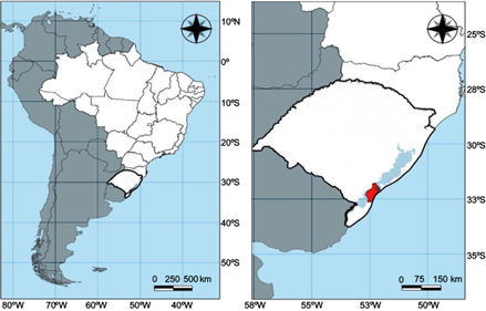
Fig. 1 Geographic location of Rio Grande city (red area in the map). Emphasis is made on the water bodies that border this region (blue areas in the right panel). To the north of the city is the Patos Lagoon, and to the south part of the Mirim Lagoon.
Parameters such as wind direction and intensity, sea currents, and seawater temperature have peculiar characteristics in the region, which greatly contribute to the formation and longer duration of fog in that location. Calm or weak winds favor the formation of radiation fog. Advection and radiation-advection fogs are also strongly dependent on wind intensity (in this case, moderate) for their formation since it occurs from the displacement of air over a relatively cooler surface. Additionally, wind speed is also an important parameter in determining fog thickness, as well as it is a decisive factor for fog dissipation. Sea currents favor the transport of colder or warmer waters to a given region. Some types of fog depend on the difference between air and surface temperature over which the air travels. In the formation of phenomena over a liquid surface, the currents can act significantly, contributing to the formation of a gradient between the air and the water temperature in the area. Therefore, it is noticeable that the location of the study region, bordered by bodies of water, influences several aspects relevant to fog formation and it is an important factor to understand the occurrences of the phenomenon.
3. Methodology
3.1 Meteorological and oceanographic data
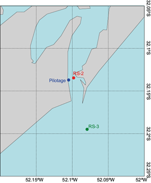
This study was developed by using meteorological data and navigation conditions observed by the Rio Grande pilotage station. Moreover, meteorological and oceanographic data were obtained from buoys of the Brazilian Coast Monitoring System project (SiMCosta). Table I shows the meteorological variables used, and Figure 2 shows the observation points considered in this study.
Table I Data used to characterize the fog occurrence in Rio Grande.
| Data | Data source | Variables | Period |
| Meteorological Station | Pilotage | Wind speed and direction, air temperature, precipitation | 01/01/2007 to 08/28/2019 |
| Rio Grande’s pilotage conditions | Navigation conditions | 04/22/2004 to 08/28/2019 | |
| Buoy RS-2 | SiMCosta Project | Wind speed and direction, air and water temperatures | 02/11/2019 to 01/16/2020 |
| Buoy RS-3 | Air and water temperatures | 02/21/2019 to 10/12/2019 |
Information about navigation conditions in the Rio Grande strip is categorized as follows: “Practical”, “Impracticable”, “Practical in analysis” and “Impracticability in analysis”. This classification is associated with the maneuvering activities of the ships in Rio Grande port region. It is presented together with the reason that caused changes in the navigation conditions. Thus, from these records, it is possible to identify the fog events that affected pilotage activities. It is worth mentioning that this is a subjective record since the change in navigation conditions is carried out by the Port Authority when some phenomenon affects the maneuver of ships. It depends on the location within the port area, the type of maneuver to be performed at the moment of the record, as well as the scope of the phenomenon that is affecting the activity.
In this study, a survey was made of events in which there was a change in navigation and maneuvering conditions due to visibility restriction. It is noteworthy that, despite the definition of fog establishing that the decrease in horizontal visibility is less than 1000 m, the records of the Rio Grande pilotage station consider a situation in which the horizontal visibility is less than 500 yards (approximately 457 m) as “Impracticable”. Therefore, the fog events considered in this work are associated with a significant visibility restriction, known as dense fog (Goswami and Sarkar, 2017).
Days in which the fog occurrence was observed concomitantly with precipitation were discarded from our analysis since, under these conditions, the visibility restriction could be associated with the precipitation. We assume that precipitation corresponds to falling water particles in the atmosphere, and it differs from the fog definition, which is water particles suspended in the atmosphere, near or close to the surface (WMO, 2017). Therefore, the cases in which low visibility was reported together with records of precipitation rate equal to or greater than 0.4 mm h-1 were discarded from our analysis. This limit value was assumed since the record of 0.2 mm h-1 could be associated with condensation of the fog over the rain gauge, which has 0.2 mm of precision. This analysis allowed us to keep 241 fog events to be analyzed.
Analyses were then carried out to verify the monthly frequency of fog occurrence at Rio Grande, as well as to quantify the total number of events, days, and hours in which the visibility affected the pilotage activities.
3.2 Numerical modeling
3.2.1 WRF model configuration
In this work, WRF v. 4.1 was used to perform simulations. The domain adopted is presented in Figure 3, which consists of three grids, with domains 02 and 03 nested from domain 01, using the one-way nesting method. It is noteworthy that domains 01 and 03 are centered in the coordinates of the Rio Grande pilotage control tower, where the main meteorological station used in this study is located. The horizontal resolution for domains 01, 02, and 03 is 9, 3, and 1 km, respectively.

Fig. 3 Domains layout used in the WRF simulations. The color shade refers to topography (in meters).
The vertical configuration of the model is very important to study phenomena in the boundary layer, such as fog. There are two relevant parameters in this configuration: the vertical resolution, and the height of the first level of the model (Tardif, 2007; Philip et al., 2016).
The lowest vertical level of the model (z1) is part of the configuration of vertical resolution in the lower part of the atmosphere. It plays a very important role in the resolution of processes near the surface (Yang et al., 2019). The definition of a thin layer near the surface requires a higher vertical resolution in the lower model layers, which will allow a better solution for the physical processes inherent to the interactions between the surface and atmosphere (Shin et al., 2012).
In this study, we assess the impact of changing the number of vertical levels and the altitude of the first model level, simulating a fog event in Rio Grande, with three different configurations. In the first configuration, we used 33 vertical levels, and the first level height was 50 m. In the second one, we configured the WRF model with 50 vertical levels, and the altitude of the first level was 20 m. In the last one configuration, we changed the first level’s model to 10 m, keeping 50 vertical levels. The Lambert Conformal Conic projection was used, due to its better suitability for the study area. The initial and lateral conditions are obtained from the analyses of the NCEP/Global Data Assimilation System (GDAS/FNL), with a horizontal resolution of 0.25º, since our objective is evaluating the ability of the WRF model to simulate dense fogs. Therefore, we chose to use analysis data instead of operational predictions from the global atmospheric model. Additionally, it is noteworthy that the model was initialized with a spin-up time of 24 h and configured with a time step of 45 s for domain 1. The physics parametrization schemes selected are shown in Table II.
Table II Physics parametrization schemes selected to perform simulations with the WRF model.
| Process | Physical scheme |
| Long wave radiation | Rapid Radiative Transfer Model (RRTM) |
| Short wave radiation | MM5 (Dudhia) |
| Surface layer | Revised MM5 similarity theory |
| Land surface | Noah land surface model |
| Cumulus | Kain-Fritsch |
| Planetary boundary layer | Yonsei University (YSU) planetary boundary layer |
| Microphysics | WRF Double-Moment 6-class (WDM6) |
According to Steeneveld et al. (2015), the boundary layer physics parameterization proved to be crucial for a better prediction of fog formation. Moreover, the microphysics scheme presented itself as an important element in the prediction of the phenomenon’s dissipation. These authors found that the dual-momentum microphysical scheme (WDM6) showed a better performance compared to the single-momentum scheme. The WDM6 scheme has as prognostic variables, besides the water mass content in its various phases, the concentrations of cloud and rain drops. This scheme is sensitive to the concentration of condensation nuclei, including their advection processes (Skamarock et al., 2019).
The YSU planetary boundary layer scheme has, among its specifics, a term of vertical mixing driven by radiative processes that is important for the life cycle of stratiform clouds, including fogs (Skamarock et al., 2019). Yang et al. (2019) evaluated previous studies and highlighted that the modeling of the formation and evolution of advective fogs is more sensitive to planetary boundary layer schemes than microphysics schemes. These authors pointed out the YSU scheme as one of the most skillful for fog prediction.
3.2.2 Horizontal visibility estimates
Horizontal visibility is the main parameter to assess fog occurrence. In addition to observation, there are some empirical methods for estimating this parameter, and, consequently, indicate the presence of fog. The visibility estimation methods evaluated in this study will be described as follows.
Kunkel (1984) proposed an estimate of visibility, in kilometers, based on the liquid water content (LWC), from the empirical relationship presented in Eq. (1).
where LWC is the liquid water content in g m-3. In this work, we use the same adaptation indicated by Fita et al. (2019) to estimate the visibility from the WRF model by using Kunkel’s method.
There are also methods that consider simpler observational parameters to compute horizontal visibility, such as the one developed by the Forecast Systems Laboratory (FSL) (Doran et al., 1999). The FSL visibility method (Eq. [2]) uses air and dew point temperatures, and relative humidity to estimate the horizontal visibility in miles.
where T and Td are the air and dew point temperatures in ºC, respectively, and RH is the relative humidity in %.
Another parameter used in this study to evaluate fog occurrence is the empirical method named Fog Stability Index (FSI). This method was developed in Germany in the 1970s and indicates the probability of radiation fog occurrence (Freeman and Perkins, 1998). Thus, different from the other methods, it is not a visibility estimation. The index is computed by using Eq. (3).
where T sfc and Td sfc are the air and dew point temperatures near the surface (usually replaced by 2 m temperature above the surface) in ºC, T 850 is the air temperature at 850 hPa in ºC, and U 850 is the wind speed at 850 hPa in kt.
FSI values greater than 55 indicate a low probability of fog occurrence. Values between 55 and 31 indicate moderate probability, and values lower than 31 indicate a high probability of radiation fog occurrence in a locality. Holtslag et al. (2010) show that the FSI highlights the conditions favorable to radiation fog formation: high humidity, stability, and low wind speed.
3.3 Study cases
After identifying the fog events in Rio Grande, four periods were selected in which the formation and maintenance of the phenomenon were observed in the port region (Table III). In the time intervals selected, there was an alternation between navigation conditions, with periods of intense visibility restrictions, where the horizontal visibility was lower than 457 m, and others with a visibility improvement, allowing navigation maneuvers to be retaken. Note that the pilotage classification information does not imply that the fog was completely dissipated. Actually, the situation described as “Practicable” minimally denotes the absence of a dense fog in the Rio Grande Port region.
Table III Detailed description of navigation conditions during the visibility restriction events selected for this study. The date and time information is in local time (GMT-3).
| Period (simulation time interval) | Start (date and local time) | End (date and local time) | Navigation condition |
| A (07/15/2019 09:00-07/18/2019 21:00) | 07/16/2019 23:30 | 07/17/2019 13:30 | Impracticable |
| 07/17/2019 13:30 | 07/17/2019 20:30 | Practicable | |
| 07/17/2019 20:30 | 07/18/2019 03:00 | Impracticable | |
| B (08/27/2019 09:00-08/28/2019 21:00) | 08/28/2019 07:00 | 08/28/2019 11:15 | Impracticable |
| C (06/17/2018 09:00-06/20/2018 09:00) | 06/18/2018 00:00 | 06/18/2018 15:00 | Impracticable |
| 06/18/2018 15:00 | 06/19/2018 00:30 | Practicable | |
| 06/19/2018 00:30 | 06/19/2018 05:00 | Impracticable | |
| 06/19/2018 05:00 | 06/19/2018 18:15 | Practicable | |
| 06/19/2018 18:15 | 06/19/2018 22:30 | Impracticable | |
| D (08/07/2019 09:00-07/10/2019 21:00) | 07/09/2019 03:00 | 07/09/2019 09:30 | Impracticable |
| 07/09/2019 09:30 | 07/09/2019 23:30 | Practicable | |
| 07/09/2019 23:30 | 07/10/2019 10:00 | Impracticable |
The study case of period A (see Table III) was used to define the best vertical configuration of the WRF model. Next, all the other cases were simulated with the model’s configuration described previously and used to analyze the ability of the model to detect the beginning, intensity, and duration of the fog. It is important to emphasize that, among the four simulation periods, the results of periods A and B will be presented in detail in this work in sections 4.2 and 4.3.
Additionally, to perform a better analysis of these study cases, observed data from the pilotage meteorological station were used together with data from the buoys of the SiMCosta Project, synoptic charts from the Brazilian Navy Hydrographic Center (CHM), and satellite images containing a tool that is able to highlight fog events, developed by the Environmental Satellites Division from the Brazilian National Institute for Space Research (DSA/INPE).
The last step is computing some statistical parameters to evaluate quantitatively the ability of the WRF model to identify dense fog occurrences. To evaluate the model performance, contingency tables are used, comparing hourly observations of dense fog occurrence, from pilotage navigation conditions, with the parameters used in this work to characterize the dense fog, i.e., the horizontal visibility computed by using FSL’s and Kunkel’s methods, beside FSI. It is noteworthy that the evaluation of the FSI took place in a different way since this parameter does not provide visibility outputs, it only indicates the probability of fog formation. For this index, we considered a fog occurrence when the values indicated a high probability of fog formation (FSI < 31). The statistical metrics evaluated are accuracy or proportion correct (PC), threat score (TS) or critical success index (CSI), odds ratio (Θ), bias, false alarm ratio (FAR), hit rate (HR), and probability of false detection (POFD) (Wilks, 2006). From the four study cases evaluated, a total of 244 h of fog simulation is considered in this analysis.
4. Results
4.1 Characterization of fog frequency in the study region
Between April 2004 and August 2019, 241 records of changes in the operating conditions of Rio Grande Strip due to the reduction of horizontal visibility to less than 500 yards, were identified. In terms of time duration, the restricted visibility impacted the port activities during 1444 h and 6 min.
The highest frequency of days affected by dense fog events in Rio Grande city, for a period of approximately 15 years, occurred in austral wintertime, between the months of May and September, with maximums in June and July. This result is in accordance with that observed by Reboita and Krusche (2000) in previous years.
4.2 Fog event case study via numerical modeling - Period A
The fog event evaluated in this section comprises an interval between July 16 and 18, 2019 (period A from Table III). The fog began to affect pilotage activities at 23:30 LT on the 16th, and the evaluation period extends until 13:15 LT on the 18th, with some intervals where it was possible to perform maneuvers. It is reiterated that impracticality records occur in situations of visibility below 457 m (500 yards) and they are subjective. Thus, it is not possible to accurately inform the start and end times of the phenomenon.
Next, results obtained from data observed during the occurrence of fog are presented, as well as a discussion of the performance of the WRF model in simulating this event, and evaluating the vertical resolution of the model.
4.2.1 Observational assessment
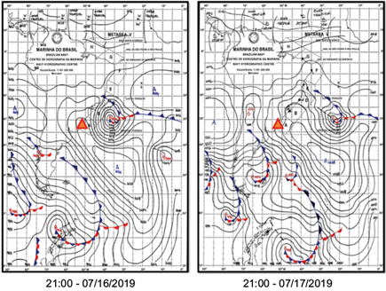
The synoptic chart analysis shows that the study region was close to the edge of a high-pressure system during the case study time interval (Fig. S1 in the supplementary material). This configuration favors the occurrence of northeasterly (NE) winds in the region. Moreover, it is worth mentioning that the influence of high-pressure systems, especially in its most central area, is a favorable factor for fog formation by radiative cooling since this synoptic system is associated with clear sky conditions and calm or weak winds. This synoptic pattern also favors the upwelling of cooler water along the coast, which can contribute to fog occurrence.
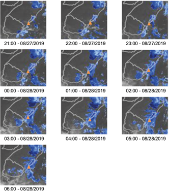
Satellite images indicated the presence of low clouds over the region of interest for this study since the early morning of July 17 (Fig. S2). Advancing in time, it is possible to verify the phenomenon evolution through the increase in low cloud cover near the estuarine area of the Patos Lagoon on the night of the 17th. From the first hours of the early morning of July 18, there are indications that the phenomenon has acquired a dynamic aspect, moving towards the south/southeast (S/SE) to the extreme south of the Rio Grande do Sul state.
The data observed during the occurrence of the phenomenon at the pilotage station and at the RS-2 buoy, from the SiMCosta project, are shown in Figure 4, where the time intervals highlighted in gray refer to the times in which the “Impracticability” condition was reported, i.e., in the period corresponding to the dense fog occurrence.
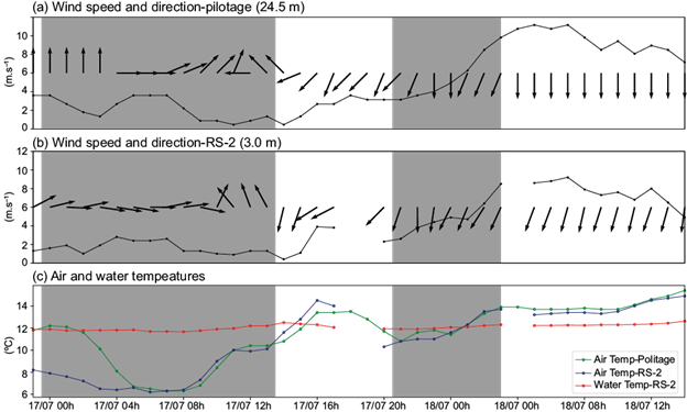
Fig. 4 Time series of wind direction and intensity at (a) the pilotage station, and (b) the RS-2 buoy. (c) Time series (local time) of air and sea surface temperatures observed during the fog event that occurred between July 16 and 18, 2019. The intervals highlighted in gray correspond to the times when the “Impracticability” condition was reported.
At the beginning of the visibility restriction, the occurrence of light winds from the south quadrant was observed. This condition may have contributed to a moisture inflow from the ocean towards the pilotage station and RS-2 buoy, favoring the formation of fog. From the afternoon of July 17, the wind changes to a northerly component, which could have initially contributed to a momentary weakening of the fog density together with the increasing air temperatures. However, the impracticable conditions returned on the evening of July 17, at the same time in which an increase in wind speed and a decrease in air temperatures were observed. Thus, the fog intensification coincides with the moment where the air temperatures recorded became lower than the sea water temperature, which suggests a transport of colder continental air over the region, providing an increase in relative humidity within the study area and re-intensifying the fog. It is noteworthy that the northeasterly winds in the study region can also contribute to channeling moisture from the Patos Lagoon towards Rio Grande city. Finally, it is observed that a few hours after the air temperatures became higher than the sea water temperature in the early morning of July 18, together with the wind intensification, there was a return to the practicable condition, which implies a better visibility condition.
An important aspect to be highlighted is that the wind direction observed at the pilotage station matches the evidenced displacement of clouds detected by the satellite product, indicating that the fog moved according to the predominant wind direction in the region. This aspect, together with the observed moderate winds, is indicative of the advective character of the phenomenon at that stage of its development.
All these factors pointed to the possibility that the fog event evaluated in this study case was a radiation-advection fog formed from a cooling process by radiative loss (radiation fog), and acquiring a dynamic aspect at a certain stage of its life cycle. From this moment onwards, the fog/low cloud was advected over a liquid surface cooler than the overlying air, following the direction of the local wind.
4.2.2.1 Vertical resolution
Considering the importance of the WRF model’s vertical configuration to simulate fog events, we assess three vertical configurations for the study case A: (i) test 1, 33 vertical levels, and the first model level height at 50 m; (ii) test 2, 50 vertical levels, and the first model level height at 20 m; (iii) test 3, 50 vertical levels, and the first model level height at 10 m. Figure 5 shows the simulated time series of meteorological variables for each vertical configuration. For this analysis, the grid point from domain 3 (closest to the Pilotage meteorological station) is used. The blue lines represent the variables simulated by the WRF with the configuration of test 1, the green ones refer to test 2 and the red ones correspond to test 3. The time intervals highlighted in gray correspond to the times when the “Impracticability” condition was reported.

Fig. 5 Time series of (a) wind at 10 m, (b) relative humidity at 2 m, (c) air temperature, (d) liquid water content, (e) mixing ratio, (f) FSI simulated by the WRF model for the grid point closest to the pilotage control tower from test 1 (in blue), 2 (in green), and 3 (in red) configurations, (g and h) visibility estimates simulated by the WRF model for the grid point closest to the pilotage control tower from test 1 (in blue), 2 (in green) and 3 (in red) configurations. The interval highlighted in gray corresponds to the times when the “Impracticability” condition was reported.
In general, WRF model simulations using the three vertical resolution configurations are in accordance with observed data of wind speed (Fig. 5a) and temperature (Fig. 5c). Although a few differences between the curves of the simulations and observed data of these variables can be noted, all simulations indicate well the behavior of wind speed and temperature, with an increase of wind speed from the afternoon of July 17, as well as higher temperatures on July 18, as compared with the 17th. The observed data of other meteorological variables are not available, however, they are used to characterize and indicate the dense fog occurrence.
The relative humidity simulated in test 1 delays to arrive at 100% when compared with the results of tests 2 and 3 (Fig. 5b). This delay, together with lower values of LWC during the early morning of July 17 (Fig. 5d) can impact the dense fog detection using a smaller vertical resolution of the model. The simulated time series of LWC and water vapor mixing ratio (Fig. 5d, e) analyzed together illustrate well the process of converting water vapor into liquid water. A process of increasing liquid water content was initiated, accompanied by a subtle downward trend in the mixing ratio variable across all tests. However, as observed for relative humidity, test 1 shows a tendency to lag this conversion compared to the other tests.
Between the parameters used to indicate dense fog occurrence, the FSI (Fig. 5f) showed promising results from the point of view of fog forecast in Rio Grande. The index was sensitive to the presence of the phenomenon, indicating a high probability (FSI < 31, dashed orange line) of fog formation in the region throughout practically the entire duration of the event, and the three vertical resolution configurations presented equivalent results for this parameter. Kunkel and FSL horizontal visibility estimates were evaluated (Fig. 5g, h, respectively). The 1 km threshold was evidenced in the time series of such parameters (solid black line) in order to perceive the time intervals that the model identified in its simulations of fog presence in the region of interest. In addition, it is noteworthy that the generated black line denotes the 500 m visibility threshold, perceiving the periods in which the WRF simulated more intense visibility restrictions, as recorded by the navigation condition data. The horizontal visibility estimated by using Kunkel’s method presented failures due to its computation being dependent on the LWC, which has values very close to 0. Taking the period in which it was possible to calculate this parameter, a relative sensitivity to what was described by the navigation conditions is noted. In all tests, this parameter pointed to visibility values below 500 m and showed a tendency towards increased visibility during the studied event. On the other hand, the FSL estimate does not depend on the LWC data. This variable showed relevant results (Fig. 5h). As previously verified, test 1 showed a delay in the characterization of the dense fog event. That is, tests 2 and 3 identified visibility values lower than 1 km from the night of July 16, while test 1 only in the early morning of July 17. All vertical configurations evaluated in this study were able to identify the presence of fog from this estimate. However, tests 2 and 3 performed better than test 1, both in characterizing the intensity of the event and in relation to formation time. Test 2 showed values close to 500 m during almost the entire interval between the night of July 16 and tthe he dawn of July 18, while test 3 was the only one that showed visibility below this threshold. All the tests were able to coherently represent the return to “Practicability”, since they indicated an increase in visibility from the early hours of July 18.
The analysis of these results showed that the increase in vertical resolution, combined with a reduction in the height of the first level of the model, produced an early formation of fog at the evaluated point. This aspect represents an improvement in the characterization of the study phenomenon since it is more consistent with the observational record. Additionally, the height of the first level of the model had a potential influence on the assessment of the intensity of the visibility restriction associated with the phenomenon, with lower values of this parameter associated with a more restricted visibility simulation. From this analysis, we adopted the vertical resolution configuration from test 3 to all other simulations performed with the WRF model. This configuration resulted in a considerable vertical discretization of the atmosphere in its lower portion, with 13 levels below 1000 m, being five below 100 m (10.0, 23.0, 39.7, 61.4, and 89.4 m). Considering that, by definition, fogs are stratiform clouds that form on the surface and have vertical extensions from a few meters up to hundreds of meters (WMO, 2017). The vertical resolution proposed in this study includes three vertical levels in the first 50 m of height, which allows a better representation of the vertical structure even in cases of shallow fogs (Román-Cascón et al., 2015).
4.2.2.2 Meteorological fields
In this subsection some variables predicted by the WRF model will be shown. The physics parameterizations used in the simulation are those presented in Table II. Only variables/fields from domain 3, which has a horizontal resolution of 1 km, will be presented in this work since they are considered more significant in terms of the results. Additionally, representative times of the fog formation and dissipation stages were selected to be discussed. The selected times are based on the pilotage station records: 23:00 LT on July 16, and 03:00 LT on July 18, 2019. Figures 6 and 7 show the fields of liquid water content (a), and water vapor mixing ratio (b) at the first vertical level of the model (located at a height of 10 m), relative humidity at 2 m, and wind at 10 m (c), air temperature at 2 m (d), and the horizontal visibility estimates by the FSL (e) and Kunkel’s (f) methods. The red dot highlighted in all figures represents the location of the pilotage weather station.
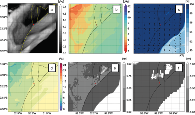
Fig. 6 Fields of (a) liquid water content, (b) water vapor mixing ratio, (c) relative humidity at 2 m together with 10-m wind, (d) air temperature at 2 meters, and (e, f) visibility estimate computed from FSL and Kunkel methods, respectively, simulated by the WRF model for July 16, 2019 at 23:00 LT.
The simulation indicates that at the closest time to the initial record of intense visibility restriction (23:00 LT on July 16, 2019), the WRF model was able to detect the presence of liquid water and high humidity values near the surface (Fig. 6), pointing out a configuration favorable to fog occurrence in the study region. In addition, the cooling process that possibly gave rise to the studied fog was evidenced. This process can be verified through the detection of a region on the continent with minimum values of water vapor mixing ratio coinciding with higher values in the field of liquid water content, which represents a conversion from water vapor to liquid water occurring in the study area, as discussed in section 4.2.2.1. The predominance of the simulated low-intensity winds, from the south quadrant, is in agreement with the observed data. Moreover, the model represents well the relative humidity with values between 99 and 100% in the fog occurrence region.
The visibility fields calculated with the variables simulated by the WRF model identify the presence of fog in the study region at the same time at which the event begins (Fig. 6). Both the FSL and Kunkel visibility estimates (Fig. 6e, f, respectively) characterized the occurrence of dense fog with visibility restriction below 500 m, in agreement with the pilotage observational record. It is noteworthy that the visibility restriction simulated by using the Kunkel method (Fig. 6f) was even more intense than that computed from the FSL method (Fig. 6e) in most areas of domain 3, at this analyzed time.
On July 18 at 03:00 LT the navigation condition returned to “Total practicability”. At this time, the WRF model was able to simulate meteorological conditions favorable to dissipate the phenomenon, as can be evaluated in Figure 7. There are no high values for liquid water content over the pilotage area, although values above 1g kg-1 were still identified over the ocean, farther from the coast (Fig. 7a). An intensification of the wind could also be observed during the early morning (Fig. 7c), which is consistent with what was observed in the meteorological station. The elevation of temperatures was also well indicated by the simulation (Fig. 7d), while no significant changes in the water vapor mixing ratio were observed over the pilotage area.

The horizontal visibility, computed by using both Kunkel and FSL parametrizations, increased over the pilotage area. Values higher than 500 m show that the model captured correctly the practicability condition at 03:00 LT on July 18 (Fig. 7e, f). The visibility fields are similar for the oceanic area; however, they present some divergences in the continental portion and in the access channel to the Patos Lagoon. The horizontal visibility estimate using the FSL method identified the presence of fog over an area larger than that derived from the Kunkel method. On the pilotage point, the FSL field still shows visibility between 500 and 750 m, while the Kunkel field no longer represents fog in the region.
The suitability of the WRF model in simulating the fog from this study case is also confirmed by its ability to simulate the dissipation of the phenomena. Both the meteorological variable fields and the visibility estimates in times after 03:00 LT (figures not shown), when the “Practicability” condition was already well characterized, are well represented, confirming the fog dissipation.
4.3 Fog event case study via numerical modeling - Period B
4.3.1 Observational assessment
Between the night of August 27 and the morning of August 28, 2019, the region of interest was under the influence of a high-pressure system (Fig. S3). This configuration is promising for fog formation by the cooling mechanism since it is related to light winds and clear sky conditions. It is also noteworthy that the city of Rio Grande was located near the edge of this system. Such positioning may favor northeast winds in the region. As of early morning on August 28, 2019, the evaluated satellite product identified the presence of low clouds in the estuarine region of Patos Lagoon (Fig. S4).
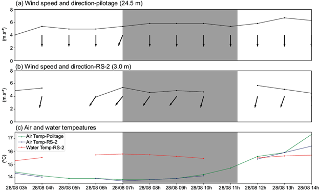
The data observed at the pilotage meteorological station and at the RS-2 meteoceanographic buoy highlighted the occurrence of light to moderate winds and throughout the interval between dawn and early afternoon on August 28, 2019 (Fig. 8). The predominance of winds from the north quadrant was evidenced in this area. In general, less intense winds were verified on the buoy in relation to the pilotage meteorological station. This characteristic may be associated with the difference in height between the two wind sensors. Another point to be characterized is the observation of air temperature lower than the water temperature during the visibility restriction. After the end of the event, this behavior reverses.
The fog event that occurred during period B presents additional information obtained from the local observations and photographic records in this interval. Noteworthy is the record of fog in the central area of the city of Rio Grande since the early morning of August 28 and the information that the maneuver prevented from taking place due to the presence of the phenomenon consisted of the entry of a ship into the access channel to the port of Rio Grande.
4.3.2 Numerical modeling assessment
Figure 9 shows the temporal evolution of the meteorological variables simulated by the WRF model at the closest grid point to the location of the pilotage meteorological station. Compared to the observed data (black lines in Fig. 9a, c), the WRF performed well in representing the meteorological variables within the study region.

Fig. 9 (a) Time evolution of wind direction and intensity at 10 m, (b) relative humidity at 2 m, (c) air and dew point temperatures at 2 m, (d) liquid water content, (e) water vapor mixing ratio (e), (f) Fog Stability Index (FSI), and (g, h) visibility estimates from Kunkel and FSL methods, respectively. Parameters are simulated by using the WRF model for the fog event that occurred on August 28, 2019. The interval highlighted in gray corresponds to the times when the “Impracticability” condition was reported and the red and green dashed lines in (g) and (h) highlight the visibility thresholds of 1 km and 500 m, respectively.
According to what was observed in the study area, the fog began its formation in the early morning of August 28, 2019. It is noteworthy that the WRF simulated favorable conditions for the presence of fog in the region from the first hours of the same day, such as the presence of light winds and relative humidity equal to or very close to 100% (Fig. 9a, b). In addition, the FSI and the visibility estimates also characterized the presence of dense fog at the evaluated point throughout the analyzed interval (Fig. 9f, g, h).
The time series of LWC and mixing ratio analyzed together indicate a dissipative process of the fog, where the variables presented opposite trends at the end of the “Impracticability” period (Fig. 9d, e). Thus, a reduction in LWC associated with increases in mixing ratio in the study region indicates a conversion of liquid water into water vapor. This characteristic may be associated with the fog dissipation process and was well represented by the WRF model.
At 01:00 LT on August 28, 2019 (the time closest to the first observational record of the fog event), the meteorological fields indicated the presence of the phenomenon (Fig. S5). The “Impracticality” interval recorded during period B occurred between 07:00 and 11:15 LT on the same day. Thus, the following fields are representative of the WRF model simulations for the start time of the intense visibility restriction event (Fig. 10).

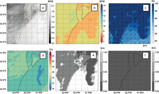
Fig. 10 Fields of (a) liquid water content, (b) water vapor mixing ratio, (c) relative humidity at 2 m together with 10 m wind, (d) air temperature at 2 m, and (e, f) visibility estimate computed from FSL and Kunkel methods, respectively, simulated by the WRF model for August 28, 2019, at 07:00 LT.
At 07:00 LT, the processes of cooling and converting water vapor into liquid water close to the surface remained highlighted by the simulations (Fig. 10a, b, d). High values of relative humidity and light and northerly winds were also evidenced (Fig. 10c).
The fields of visibility also characterized the “Impracticability” condition, showing horizontal visibility restrictions for 500 m or less in the study area (Fig. 10e, f). A relevant aspect to highlight is the evolution characterized by the FSL visibility estimate (Fig. 10e), which identified visibility values of 250 m or less over the ocean, very close to the entrance of the access channel to Patos Lagoon. This characteristic was shown in accordance with the report of visibility conditions by the ship unable to access the channel and which was waiting on the high seas for favorable navigation conditions. The fog characterized by the Kunkel method (Fig. 10f) showed greater spatial extension and was more intense than that described by the FSL methodology (Fig. 10e).
At 11:00 LT on August 28 (the moment closest to the return to the “Practicability” condition), the WRF model pointed to indications of the beginning of the dissipative process of the fog evaluated in the study area. From Figure 11 it is possible to perceive a slight acceleration of the winds in the region, as well as a reduction in the area of maximum relative humidity. Furthermore, the cooling process and the mechanism for converting water vapor into liquid water (Fig. 11a, b, d), characteristic of the formation and development of some types of fog, were not evident.

Both visibility estimates pointed to a reduction in the area covered by fog at this stage of its life cycle, despite still featuring visibility conditions equal to or less than 500 m in the vicinity of the estuarine region of Patos Lagoon (Fig. 11e, f). In this way, the WRF showed the ability to detect the beginning of the dissipative process of this phenomenon.
It is noteworthy that, from the field of visibility FSL (Fig. 11e), it was possible to perceive the absence or dissipation of fog over the ocean, indicating better navigation conditions at the entrance of the access channel to the port region of Rio Grande. Based on the knowledge of the type of maneuver to be carried out immediately after returning to “Practicability” (ship entry), it was possible to assess that the WRF model performed well in this characterization.
4.4 Statistical analysis
The results obtained for the statistical analysis of the performance of dense fog simulations based on the WRF model will be presented in this section. It is reiterated that, in this evaluation, the hourly outputs of the four simulations described in Table III were considered, totaling 244 h.
From Table IV, it is possible to verify that the FSL visibility estimate proved to be the parameter with the best statistical metrics aimed at verifying the forecast of fog occurrence, followed by Kunkel’s visibility estimate. The two estimates showed similar results for several statistical metrics, being slightly higher in view of the prediction of the phenomenon for the FSL estimate. The results combine a significant rate of correct predictions and probability of detection of the phenomenon, as well as the lowest rate of false alarms and low probability of false detection. In addition, they present a bias slightly higher than 1, indicating a small overestimation of the number of hours of occurrence of dense fog. It is also noteworthy that the fog forecast by the WRF model based on the FSL estimate presented a higher odds ratio than the other evaluated parameters, thus being able to be characterized as the most accurate forecast.
Table IV Statistical metrics for forecasting dense fog in Rio Grande from the WRF model.
| Metric | FSL | Kunkel | FSI |
| PC | 0.71 | 0.70 | 0.38 |
| TS | 0.42 | 0.39 | 0.29 |
| Θ | 7.18 | 5.53 | 3.14 |
| Bias | 1.58 | 1.55 | 3.18 |
| FAR | 0.52 | 0.54 | 0.70 |
| HR | 0.76 | 0.71 | 0.94 |
| POFD | 0.30 | 0.31 | 0.83 |
The best results for each statistical metric are highlighted in bold.
In this study, the best outcomes for the accuracy or proportion correct (PC), threat score (TS), and hit rate (HR) assume the value closest to 1. For false alarm ratio (FAR) and probability of false detection (POFD), the best result obtained is characterized by proximity to 0. The highest odds ratio (Θ) value features the most accurate prediction. Regarding the bias, the best result is 1. Values above 1 indicate an overestimation, and values below indicate an underestimation of fog occurrence.
Despite having the highest probability of event detection, the FSI was also associated with a high false alarm rate and a significant probability of false detection. This characteristic points to an overestimation of the forecast of fog by this index or predominance of identification of high probabilities of the occurrence of the phenomenon.
5. Conclusions
In the present work, we aimed to evaluate the ability of the WRF model to simulate dense fog events in Rio Grande city, southern Brazil. A brief characterization of the fog occurrence and frequency in this study region was also carried out.
The 15-year data period indicated that the highest occurrence of fog in the study region was between May and September, with a maximum frequency in June and July, which is in accordance with previous studies.
A sensitivity test was performed to assess the impact of the WRF model’s vertical resolution in detecting a dense fog. The results showed that the increase in the number of vertical levels, combined with a reduction in the height of the first level of the model, can improve its ability to simulate the fog formation processes since the atmospheric vertical structure can be better represented.
The analysis of dense fog events that occurred in Rio Grande city is made by using meteorological observed data, synoptic charts, and satellite images, besides the simulation with the high-resolution WRF model, adequately configured. The observational analysis of the phenomenon allowed to identify that a high-pressure system influenced the meteorological conditions in the study region. Moreover, some relevant characteristics of fog formation were observed and confirmed, such as calm or weak wind conditions and air temperature lower than the seawater temperature. In addition, the study cases analyzed in this work show that dense fogs in Rio Grande can also be maintained in conditions of moderate winds when there is an increase in humidity in the pilotage station region, and an inversion of the patterns of air and seawater temperatures were observed. This last condition has pointed to a displacement of relatively warmer air over a cooler surface region, indicating a dynamic characteristic of some fogs.
The evaluation of the phenomenon from the numerical simulations showed promising results. In general, the WRF model proved to be capable of simulating and probably predicting representative fields for the formation and dissipation processes of the phenomenon studied. The time evolution of the variables analyzed was coherent with the observed data, characterizing the different stages of the event. Additionally, the FSI index showed sensitivity to the occurrence of the fog evaluated, indicating a high probability of occurrence throughout almost the whole analyzed event. Kunkel’s and FSL’s visibility estimates proved to be applicable tools to the forecast of the event, indicating intense restriction of visibility throughout the study periods and representing the trend of dissipation of the phenomenon in a coherent and clear way. Statistical analysis of the four study cases simulated by using the WRF model showed that the FSL visibility estimate proved to be the better parameter to indicate dense fog occurrence.
The results of this study suggest that the proposed high-resolution configuration of the WRF model is promising for the forecast of dense fog events. The generated fields and variables’ time evolution highlighted the model’s ability to predict the onset, duration, dissipation, and intensity of the fog cases studied. Considering the difficulty of forecasting this type of events (in particular, dense fogs with such reduced visibility) and the complexity of the region’s geography, these results are promising in the search for an operational tool that helps navigation sectors, such as the pilotage of Rio Grande, in decision-making to favor waterway safety.