


 nueva página del texto (beta)
 Inglés (pdf)
 Artículo en XML
 Referencias del artículo
 Enviar artículo por email
 Citado por SciELO
  Similares en
SciELO
Similares en
SciELO 
 Permalink
1. Introduction
Temperature and precipitation are two essential climatic variables affecting biotic and abiotic environments, and climate has a crucial effect on plant growth, and other living conditions. Knowing the spatial distribution of climate is an essential means of explaining the variation in biological activity, which is also necessary for developing stochastic models (Hutchinson, 1995). Deviations from optimum climatic conditions adversely affect plant distribution (Sáenz-Romero et al., 2010), growth, and productivity (Orlandini et al., 2009). Climate classification systems such as Thornthwaite and Koppen have proven the main effects of temperature and precipitation on plant species distribution (Attorre et al., 2007). The relationships between climate and plants are reciprocal (Rebetez and Dobbertin, 2004).
Climate factors have been used as independent variables to predict stand productivity and forest development by controlling carbon uptake, respiration loss, tree mortality, organic matter accumulation, shedding, and carbon loss (Bernier and Apps, 2006). Climatic variables are also crucial in afforestation studies. Regional climate is a fundamental determinant of plant productivity in agriculture, forests, and grasslands (Monserud et al., 2006; Yener and Altun, 2017). In addition, variables extracted from climate maps were used to predict the expansion of many bugs, such as the mountain pine beetle (Dendroctonus ponderosae Hopkins) and spruce budworm (Choristoneura fumiferana Clem.) (Bernier and Apps, 2006).
Climatic variables vary according to latitude, longitude, elevation, topography, and distance from the sea (Zhang et al., 2011). Despite their importance, weather stations in developing and undeveloped countries are insufficient due to limited budgets, inaccessibility to certain areas, and staff shortages (Taesombat and Sriwongsitanon, 2009; Samanta et al., 2012). Therefore, interpolating climate data from these stations in an inexpensive way is necessary (Shu et al., 2011; Samanta et al., 2012). However, studies whose estimates are poor and non-reproducible have been generally based on traditional knowledge and subjective considerations using observed values at adjacent stations (Tveito, 2007).
Climate surfaces refer to spatially interpolated climate data on high-resolution grids; they provide information to decision-makers and are used in many applications, including biology, environmental, and agricultural sciences (e.g., forestry and horticulture) (Hijmans et al., 2005; McKenney et al., 2013; Shan et al., 2020; Tan et al., 2021). In this context, surface resolution is essential. The higher the spatial resolution, the higher the environmental variability to capture, especially in mountainous areas, which are critical for research planning, experimental design, and technology transfer. High-resolution climate surfaces are helpful for climate change in terms of species distribution, forest plantations, and agricultural crop productivity (Cuervo-Robayo et al., 2014).
Inverse distance weighting (IDW), kriging (CoKRG), parameter-elevation regression on independent slopes model, and thin-plate smoothing spline (TPS) are among the most commonly used interpolation methods, taking into account data features, sophisticated algorithms, and accuracy, for developing climate surfaces (Attorre et al., 2007; Shu et al., 2011; Basconcillo et al., 2017). TPS and CoKRG used in mountainous areas (Shan et al., 2020) are crucial in the computational, accurate, and operationally straightforward interpolation of climate data (Hutchinson, 1995). The Australian National University spline-based software (ANUSPLIN) also uses the TPS algorithm and has the outstanding advantage of interpolation. On the one hand, a smoothing term is used to reduce cross-validation error; on the other hand, the relationships between climate variables (e.g., temperature and precipitation) and elevation can spatially change in ANUSPLIN (Ma et al., 2016). Because climate data are strongly affected by topography, this package also considers and models the effects of topography, including the horizontal and vertical coordinate systems. This technique is used to model climate data in addition to other environmental variables, for example, rainfall erosivity (Ma and Zuo, 2012), and is superior to CoKRG due to its simplicity and because it does not require prior calibration for each parameter (Guo et al., 2020).
In this study, Turkey was examined as the case study because it is a developing country with a scarce monitoring station network. Therefore, climate maps are required to obtain accurate, reliable data. By combining high-resolution climate maps with temporal dimensions, such datasets could be a critical tool for monitoring and determining global climate change and meteorological disaster risk in the country (McKenney et al., 2006; Huayang et al., 2019). Similar interpolation studies have been performed in Turkey to fulfill the needs of different methods (Apaydin et al., 2004; Bostan et al., 2012; Güler and Kara, 2014; Aydin et al., 2016; Tanir and Zengin, 2016). However, none of these studies used ANUSPLIN to model climate data, such as temperature and precipitation.
In several aspects, ANUSPLIN is better than other methodologies: (1) it has higher accuracy than local regression models, using all data points to calibrate a continuous spatially fluctuating dependency on elevation (Price et al., 2000); (3) the software also generates predicted error surfaces not provided by other methods, in addition to interpolated data (Hutchinson and Xu, 2013); (3) it is also better than satellite models in detecting the minimum and maximum values of climate data, for example, precipitation (Wang et al., 2021); and (4) it has more details and resolutions (Guo et al., 2020) and is not time-limited. For example, data from ERA40 are limited to 1957-2002. Therefore, choosing spatially explicit, dependable models such as ANUSPLIN provides decision-makers with valuable information (Lilhare et al., 2019). This information helps experts explain the impacts of global climate change on the function and distribution of terrestrial ecosystems and forecast its possible implications (Price et al., 2000).
Therefore, this study aimed to generate climate surfaces for mean annual (MAT), minimum (MAMINT), and maximum (MAMAXT) temperature, and total precipitation (MATP) by using ANUSPLIN software. The model maps were then compared with other spatial modeling methods, including IDW, CoKRG, lapse rate (LR), and multiple linear regression (MLR). Finally, the results were examined based on (1) diagnostic statistics from the surface-fitting model, such as signal, mean, root mean square predictive error (RTGCV), root mean square error estimate (RTMSE), root mean square residual of the spline (RTMSR), and estimate of the standard deviation of the noise in the spline (RTVAR); (2) a comparison of error statistics between interpolated surfaces and withheld climate data from 81 stations; and (3) a comparison with other interpolation methods, such as IDW, CoKRG, MLR, and LR, by using model performance metrics, such as mean absolute error (MAE), mean error (ME) or bias, root mean square error (RMSE), and adjusted coefficient of determination (R2 adj).
2. Material and methods
2.1 Study area
The study area was Turkey, extending between northeastern Asia and southeastern Europe, with 780 580 square km. Its coastline is 3558 km long (Fig. 1). Three seas surround Turkey: the Black Sea, the Aegean Sea, and the Mediterranean Sea, with an interior sea, the Marmara, connecting the Black Sea and the Aegean Sea through Bosphorus and Dardanelles (Paradise, 2014). The elevation in the country ranges from sea level to 5137 m, with an average of 1132 m. The summit altitudes of the plateaus increase to the eastern Anatolian highlands, connecting to the Caucasus and Zagros ranges (Kuzucuoglu et al., 2019). The climate is characterized by mountains and mountain ranges running parallel to the coast and rising from the western to the eastern parts of the country. There are four dominant climate types: the humid temperate Black Sea, continental inland, Mediterranean, and Mediterranean-like climates. These climate types are influenced by two main factors: (1) various atmospheric disturbances and weather types originating from polar and tropical regions, and (2) topography, sudden rise in elevation, land-sea interactions, and thermodynamic influences (Turkes, 2020). The average temperature is 23 ºC in summer and -2 ºC in winter, with a mean of 13.5 ºC. There were significant differences in the precipitation totals for the inner and coastal parts. For example, Rize and Hopa on the Black Sea coast receive the greatest amount of precipitation, and provinces such as Konya and Igdir received the least.

While the average annual precipitation for Turkey was determined as 574 mm by Sensoy et al. (2008), who used 101 weather stations from Turkey between 1981-2010, Bostan et al. (2012) determined it as 628.2 mm using 225 weather stations between 1970-2006.
2.2 Data
The climate data consisted of MAT, MAMINT, MAMAXT, and MATP. To obtain this data from the Turkish State Meteorological Services (MGM, 2018), 274 weather stations were used for 1960-2017. The quality and homogeneity of long-term temperature and precipitation data obtained from MGM have been systematically analyzed (Turkes et al., 2002; Turkes and Tatli, 2009; Komuscu, 2010; Arikan and Kahya, 2019). The quality of the data, such as duplication, was also checked. To develop the models 70% of the stations were used; the remaining 30% was set aside for model validation. Sample stations in the training and test data sets were randomly selected. The elevation information for weather stations was extracted from digital elevation model (DEM) data (NASA/METI/AIST, 2009) using the stations’ longitude and latitude.
Although the observation period of the stations varies slightly according to the variables measured, this period could be classified as < 30 years (6.3-7.4%), 30-40 years (8.1-8.5%), 40-50 years (12.-12.5%), and > 50 years (72.4-72.8%).
2.3 Interpolation methods
2.3.1 Australian National University Spline (ANUSPLIN)
ANUSPLIN is a Fortran spatial interpolation software package. It uses the thin-plate smoothing spline algorithm developed by Hutchinson and Xu (2013) to fit climate surfaces to noisy data as a function of one or more independent variables. This approach is well suited to interpolating noisy climate data through variable terrain and performs well compared with other techniques (McKenney et al., 2006). This package comprises programs such as Spline, Selnot, Addnot, Lapgrd, Lappnt, and Gcvgml. In addition, the package interrogates the fitted surfaces as point and grid forms while developing standard-error surfaces. This method enabled the measured data to be transferred from weather stations to the climate surface grids, and the methods determined errors on surface grids, validating the cross-validation techniques.
Thin-plate smoothing spline interpolation techniques were first introduced by Wahba (1979, 1990) and Hutchinson (1991), who first used this technique for spatial interpolation of climate data and developed the ANUSPLIN software. The model for thin-plate spline functions for N observed data values zi given by Hutchinson and Xu (2013):
In Eq. (1) f is the n unknown smooth function of x i ; z i shows the dependent variable (e.g., temperature and precipitation); x i is the independent variable, such as longitude, latitude, and elevation; y i is the p-dimensional vector of independent covariates; b is an unknown p-dimensional vector of coefficients of y i ; e i indicates zero-mean random errors, accounting for measurement error and deficiencies in the spline model, with a variance of w i σ 2 , where w i refers to the relative error variance (known), and σ 2 is the error variance (unknown), which is constant across all data points (Hutchinson, 1991; Hutchinson and Xu, 2013).
The function f and the coefficient vector b are determined by minimizing:
where J m (f) is a measure of the complexity of f (the “roughness penalty” is defined in terms of an integral of the mth order partial derivatives of f), and p is a positive number called the smoothing parameter. As p approaches zero, the fitted function may become an exact interpolant. As p approaches infinity, the least-squares with order depends on the order m of the roughness penalty.
The smoothing parameter is usually chosen by minimizing the measure of the predictive error of the fitted surface calculated via generalized cross-validation (GCV). By implicitly eliminating each data point and computing the residual from the omitted data point of a surface fitted to all other data points using the same value of p, Eq. (3) calculates the GCV for each value of the smoothing parameter p. GCV is then a suitably weighted sum of the squares of these residuals (Zhang et al., 2011; Hutchinson and Xu, 2013).
A, I, and tr (I-A) in Eq. (3) indicate the identity matrix, influence matrix, and residual degrees of freedom, respectively, whereas Eq. (4) calculates W, which is the diagonal matrix.
The variance σ 2 of the data error e i in Eq. (5) is formulated by
If σ 2 is known or estimated, an unbiased estimate of the “true” mean square error of the fitted function across the data points is provided by
Craven and Wahba (1978) have shown that under suitable conditions, the formula is
The weighted mean residual sum of squares is provided by
RTVAR, RTGCV, RTMSE, and RTMSR are obtained by taking the square roots of VAR, GCV, MSE, and MSR (Eqs. [5], [3], [6], and [8], respectively), and written to the output log files.
This study used a second-order spline with no transformation for the temperature and square root transformation for the precipitation recommended by Hutchinson and Xu (2013) to reduce positively skewed values by using ANUSPLIN v. 4.4. Only the SPLINE and LAPGRD programs were used in this study. While SPLINE fits an arbitrary number of (partial) thin plate smoothing spline functions of one or more independent variables, LAPGRD calculates values and Bayesian standard error estimates of partial thin plate smoothing spline surfaces on a regular rectangular grid.
2.3.2 Inverse distance weighting (IDW)
IDW is one of the simplest and most commonly used methods. The weighted average of data within a particular cut-off distance or from a given number m of the closest points estimates attributes at unknown points (typically 10-30) (Mitas and Mitasova, 1999; Chen and Guo, 2017). The assumption is that sampled points closer to the unsampled point are more similar in their values than those farther away (Panigrahi, 2014). The weights mentioned in this method are calculated using Eq. (9):
where d i is the distance between x 0 and x i , p is the power parameter, and n shows the number of sampled points used for interpolation. The most important factor affecting the accuracy of the method is the power parameter, which is generally set to 2. In the case of its increase, the estimation will be more influenced by samples around and the interpolation will be local, not global (Panigrahi, 2014).
2.3.3 Co-kriging (CoKRG)
The assumption in kriging is that the spatial variation in a regionalized variable is too irregular to be modeled by a mathematical function but it can be modeled by a stochastic distribution, which is based on exploring and then modeling stochastic aspects of the variable, which is similar to IDW. CoKRG uses a linear combination of weights at known points to predict values at unknown points (Beek, 1991; Wu and Hung, 2016). The co-kriging method is the multivariate equivalent of kriging, which is only applicable when multivariate data is involved (Hooshmand et al., 2011). The general equations of co-kriging estimator are;
While u shows the primary variable, v shows the secondary variable, contributing to the estimation of primary variables. The cross semi-variogram is determined before and defined by Eq. (11):
i, λ i is the weight associated with the data, µ is the Lagrange coefficient, and γ(x i , x j ) is the value of the variogram corresponding to a vector with origin in xi and extremity in x j .
2.3.4 Multiple linear regression (MLR)
MLR, calculated using Eq. (12), is a regression model that uses the relationships between the response (dependent) and explanatory (independent) variables. In the study, while mean, minimum, and maximum temperatures and precipitation were used as dependent variables, latitude, longitude, and elevation were used as independent variables.
Z(s) is the response variable at location s; β 0 , β 1 to β n are intercept terms and regression coefficients, X 1 to X n are the values of 1 to p explanatory variables, and ε(s) is the residual term at location s. The MLR model estimation is based on the least-squares method, which minimizes the sum of squares of the discrepancies between the observed and predicted values (Sheather, 2009).
2.3.5 Lapse rate (LR)
The LR, defined as the changing adiabatic cooling and warming rate in the atmosphere, was developed to predict air temperature based on the altitude above sea level. It determines the air temperature of unsampled points by using the value of the nearest weather station and the differences between the elevations of an unsampled and sampled point. The method assumes that LR is constant throughout the study area (Panigrahi, 2014). The decrease in the annual temperature in Turkey is recommended to be approximately 0.5 ºC per 100 m rising from the sea level (Erinc, 1984).
where Tp is the temperature at the unsampled location/point, To shows the temperature measured at the sampled location/weather station nearest to the unsampled point, LR is 0.5 C for Turkey in the literature, and h represents the differences between the elevations of sampled and unsampled locations in a unit of hectometer.
Similar to temperature, precipitation also increases with elevation above sea level, to some extent. This change in rainfall is also due to the LR, which promotes condensation in the air mass and thereby rain (Turkes, 2010). The increasing rainfall is calculated using Eq. (14), developed by Schreiber (1904), a Czech scientist. The annual precipitation in Turkey is approximately 40-50 mm per 100 m and is recommended to be 45 mm (Erinc, 1984).
where Ph shows the unknown (to be calculated) precipitation in unsampled locations, Po is the mean annual precipitation at the nearest sampled location (weather station), h represents the differences between elevations of sampled and unsampled locations in a unit of hectometer, and 45 is a constant defined in previous studies.
2.4 Model performance criteria
RMSE, MAE, ME, and R2 adj were used to evaluate and compare the methods. The error metrics were formulated using Eqs. [15]-[18].
Where ŷ is the predicted value of y, y̅ is the mean value of y, n is the number of observations, and k is the number of estimated parameters.
3. Results and discussion
3.1 Spatial interpolation by ANUSPLIN
Diagnostic statistics for interpolated climate data from 1960 to 2017, such as MAT, MAMINT, MAMAXT, and MATP were obtained using the SPLINE and LAPGRD tools in ANUSPLIN software (Table I). The final climate surfaces and their respective standard errors (error covariance) for precipitation and mean, minimum, and maximum temperatures were generated using 274 weather stations (70% for training and 30% for the test) distributed throughout the country.
Table I Summary statistics for annual climate surfaces obtained with ANUSPLIN.
| Statistics | Signal ratio | Min. | Max. | Mean | SD | SE | RTGCV | RTMSE | RTMSR | RTVAR | ρ |
| MAT (ºC) | 0.38 | -11.8 | 19.7 | 13.34 | 3.47 | 0.17 | 0.55 | 0.27 | 0.31 | 0.40 | 0.03 |
| MAMINT (ºC) | 0.46 | -18.9 | 16.6 | 8.04 | 3.95 | 0.29 | 0.96 | 0.48 | 0.46 | 0.66 | 0.02 |
| MAMAXT (ºC) | 0.53 | -3.4 | 26.0 | 19.41 | 3.22 | 0.18 | 0.59 | 0.29 | 0.26 | 0.38 | 0.01 |
| MATP (mm) | 0.58 | 260.8 | 2233.0 | 654.88 | 301.9 | 35.2 | 51.4 | 25.3 | 21.9 | 33.5 | 0.01 |
ANUSPLIN: Australian National University Spline; SD: standard deviation; SE: standard error; RTGCV: root mean square predictive error; RTMSE: root mean square error estimate; RTMSR: root mean square residual of the spline; RTVAR: standard deviation of the noise in the spline; MAT: mean annual temperature; MAMINT: mean annual minimum temperature; MAMAXT: mean annual maximum temperature; MATP: mean annual total precipitation.
The summary statistics for the surfaces are listed in Table I. MAT, MAMINT, and MAMAXT averaged approximately 13.34, 8.04, and 19.41 ºC, respectively. The MATP averaged approximately 654.88 mm. The minimum and maximum values from the fitted surfaces ranged from -11.8 to 19.7, -18.9 to 16.6, and -3.3 to 26.0 ºC for MAT, MAMINT, and MAMAXT, respectively, and 260.7 to 2232.6 mm for MATP (Figs. 2a and 5a). The covariance error ranged from 0.45 to 0.77 ºC for MAT, 0.72 to 1.34 ºC for MAMINT, 0.43 to 0.78 ºC for MAMAXT, and 52.9 to 470.2 mm for MATP (Figs. 2b and 5b). Figures 2b and 5b showed that the error covariances of fitted surfaces were relatively higher in the mountainous part of the eastern Black Sea and eastern Anatolia than in the rest because of an insufficient weather station network and the sudden rise in elevation resulting in spatial variability in temperature and precipitation. However, ANUSPLIN enables better prediction in such areas than other techniques, by calibrating a spatially varying dependence on elevation, which uses all data points (Price et al., 2000). Basconcillo et al. (2017) and Zhao et al. (2019) have reported similar cases in the Philippines and the Tibetan Plateau, respectively. However, Ma et al. (2015, 2016) stated that inconsistent dense weather stations and complex terrain also cause interpolation errors. Huayang et al. (2019) found a larger RMSE of 1.5 ºC in the mountainous parts of southern and western Anhui than in the other parts of the region (RMSE = 0.7 ºC). Bostan et al. (2012) found similar results, implying larger errors (336 mm) in the eastern part of Turkey than the western part (236 mm) in interpolating precipitation. Zhao et al. (2019) found an error covariance for China between 1951 and 2011 of 0.7-1.1 ºC and 8-143 mm; they also reported relatively high errors in temperature and precipitation, particularly when there were insufficient weather stations.

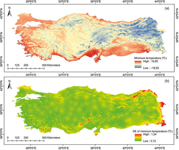
Fig. 3 (a) Interpolated surface for mean annual minimum temperature (MAMINT) and (b) its standard errors.

Fig. 4 (a) Interpolated surface for mean annual maximum temperature (MAMAXT) and (b) its standard errors.
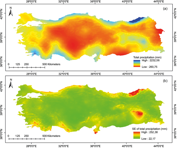
Fig. 5 (a) Interpolated surface for mean annual total precipitation (MATP) and (b) its standard errors.
Hutchinson and Xu (2013) introduced diagnostic statistics. The mean smoothing parameter ρ is nearly zero (0.01 to 0.03), indicating an exact interpolant (Hutchinson and Xu, 2013). Zhao et al. (2019) found that this smoothing parameter was 0.01-0.12 for temperature and 0.02-0.06 for precipitation. The signal, defining the number of degrees of freedom of the fitted spline for the climate surfaces, is below one half of the number of weather stations or slightly higher than it.
The signal ratio (the ratio of the signal of the fitted spline to the number of data points) ranged between 0.38 and 0.58. RTGCV, a robust measure and square root of GCV, used for the predictive performance of a climate surface, was found as 0.55, 0.96, and 0.59 ºC for MAT, MAMINT, and MAMAXT, respectively, and 51.4 mm for MATP.
The RTMSE (the estimate of the true interpolation error over the data points after measurement error in data has been removed) was 0.27, 0.48, and 0.29 ºC for MAT, MAMINT, and MAMAXT, respectively, and 25.3 mm for MATP. The RTGCV and RTMSE values from this study are consistent with those of other studies that have used ANUSPLIN to interpolate climate data. The error statistics in Table I show that the developed surfaces are good (McKenney et al., 2006; Zhang et al., 2011; Ma et al., 2016; Zhao et al., 2019; Shan et al., 2020). Zhao et al. (2019) also used ANUSPLIN to interpolate temperature and precipitation with 0.025º resolution in China from 1951-to 2011 in an area of 9 597 000 km2, using data from stations (1153 for temperature and 1202 for precipitation). They found an RTGCV, RTMSR, and RTVAR of 0.88-1.43, 0.35-0.52, and 0.58-0.69 ºC, and 1.17-3.10, 0.82-2.24, and 0.89-2.62 mm for precipitation. The spatial resolution of generated surfaces was 0.005º equaling 0.6 km. Climate maps with fine spatial resolution are very important tools for showing climatic characteristics, especially in complex terrain (Zhao et al., 2019) like in Turkey.
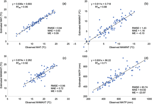
The results from the developed surfaces were also validated using test (withheld) stations. A study performed by Cuervo-Robayo et al. (2014) interpolated maximum and minimum temperatures and total precipitation in Mexico, in addition to 19 bioclimatic variables by using ANUSPLIN. The number of stations used to interpolate climate data and the resolution of maps was about 5000 and 0.008º for the study. Average RTGCV for monthly temperature and precipitation was 1.26-1.12 ºC and 24.67%, and the RTMSE was 0.48-0.56 ºC and 11.11% for temperature and precipitation. The MAE was 0.76 ºC for the minimum and maximum temperature and 8.90 mm for precipitation, and the model performance criteria are presented in . In a study to interpolate temperature and precipitation in Mexico, using ANUSPLIN, the percent RTGCV and RMSE were 8-23.5 and 3.5-23.6 for MAMINT, 5.1-6.8 for MAMAXT, and 20.0-26.8 for MATP (Sáenz-Romero et al., 2010). The coefficient of determination (R2 adj) with RMSE in this study was 0.95 with 0.8 ºC, 0.88 with 1.43 ºC, 0.92 with 0.96 ºC, and 0.71 with 83.7 mm for MAT, MAMINT, MAMAXT, and MATP, respectively. The model fit was adequate according to model statistics. MAE, RMSE, and R2 in a study (Shan et al., 2020) were 0.85, 1.06 ºC and 0.52, respectively, for the Middle East of the Qilian Mountain. Ma et al. (2017) developed rainfall surfaces with a spatial resolution of 10 × 10 km for the 9 597 000 km² in their study, using 894 weather stations. They found that the r and MSE for monthly rainfall were 0.83 to 0.89 and 25.4 to 27.8 mm, respectively, in China’s border areas.
Withheld data (approximately 30%) was also used to test the developed surfaces accuracy and the magnitudes of withheld errors (e.g., MAE and ME; Fig. 6), which were 0.63 and 0.09 ºC, 1.16 and -0.10 ºC, 0.72 and 0.05 ºC, and 54.8 and -23.97 mm for MAT, MAMINT, MAMAXT, and MATP, respectively. The percent error, ranging from 3.9 in MAMAXT to 16.6 in MAMINT, was small, slightly underestimated for MAMINT and MATP and overestimated somewhat for MAT and MAMAXT. These errors are consistent with those reported in the literature (McKenney et al., 2006; Hopkinson et al., 2012; Cuervo-Robayo et al., 2014; Ma et al., 2015; Zhao et al., 2019). For example, Cuervo-Robayo et al. (2014) determined those values for MAMINT, MAMAXT, and MATP in Mexico: 1.32 and -0.10 ºC, 1.15 and 0.04 ºC, and 15.43 and -2.25 mm, respectively.
3.2 Comparison of ANUSPLIN with other interpolation methods
The model was also validated by calculating predictive measures such as R2 adj, MAE, ME, and RMSE, using differences between fitted surfaces and withheld data, and compared ANUSPLIN with other interpolation techniques such as IDW, CoKRG, MLR, and LR. The fitted surfaces explained 95, 88, 92, and 71% of the variance in MAT, MAMINT, MAMAXT, and MATP, respectively (Fig. 6a-d). The RMSEs were 0.84, 1.43, and 0.96 ºC for MAT, MAMINT, and MAMAXT, respectively, and 83.7 mm for MATP. Many studies (McKenney et al., 2006; Hopkinson et al., 2012; Cuervo-Robayo et al., 2014; Ma et al., 2015; Zhao et al., 2019), including this one, have modeled climate data using ANUSPLIN and validated the model using data and diagnostic statistics.
3.2.1 Mean annual temperature (MAT)
All climate data were interpolated with the IDW, CoKRG, MLR, LR, and ANUSPLIN techniques and compared using performance indices such as R2 adj, RMSE, and MAE between fitted surfaces and the withholding dataset.
While the mean observed MAT was 12.39 ºC, the predicted MAT average was between a minimum of 12.39 ºC and a maximum of 12.67 ºC, belonging to ANUSPLIN and LR, respectively. ANUSPLIN accounted for 95% of the variance in MAT, with an RMSE of 0.84 ºC (Fig. 6a). As shown in Figures 6a and 7a-d, ANUSPLIN outperformed the other techniques with a higher R2 adj (0.95), as well as lower RMSE (0.84ºC) and MAE (0.63 ºC).
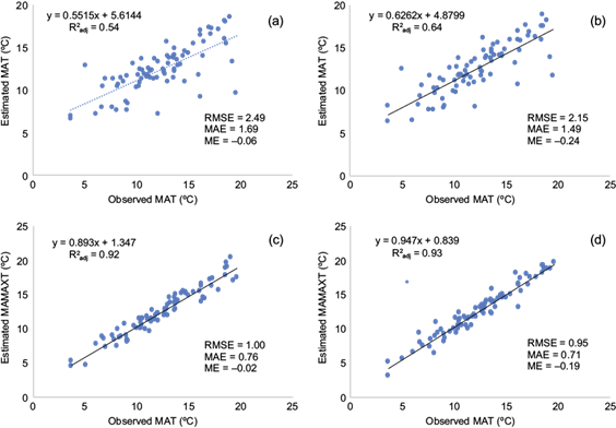
Fig. 7 Correlations and error metrics between observed and predicted MAT by interpolation methods (a) IDW, (b) CoKRG, (c) MLR, and (d) LR). (MAT: mean annual temperature; IDW: inverse distance weighting: CoKRG: kriging; MLR: multiple linear regression; LR: lapse rate).
IDW had the lowest performance and accounted for 54% of the variance in MAT, with an RMSE of 2.49, MAE of 1.69, and ME of -0.06 ºC. However, LR and MLR performed well, with a slightly lower R2 adj and slightly higher RMSE and MAE compared to ANUSPLIN ( . Other methods followed ANUSPLIN in the order of LR > MLR > CoKRG > IDW in their predictive performance criteria, except for ME, which averaged approximately-0.24 to 0.09 ºC, indicating bias; the lowest ME was achieved in the MLR method with -0.02 ºC. The independent variable common to all three top models is altitude, which strongly affects air temperature (r = -0.87) and is attributed to the LR method (Hutchinson and Xu, 2013). Many studies using ANUSPLIN for temperature interpolation (Price et al., 2000; Shu et al., 2011; Ren-Ping et al., 2016; Shan et al., 2020) have reported that it is the best technique. Unlike the findings in this study, Güler and Kara (2014) and Lilhare et al. (2019) found MLR and IDW to be superior to ANUSPLIN in studies performed in the middle Black Sea region of Turkey and the lower Nelson River basin in Manitoba, Canada, respectively. Price et al. (2000) and Shan et al. (2020) also reported a higher interpolation accuracy of ANUSPLIN with lower RMSE (0.85 ºC) compared to the gradient plus inverse distance squared (0.89 ºC) and the LR (3.57 ºC) methods for annual air temperature in BC/Alberta and the middle east of Qilian Mountain.
Demircan et al. (2011) interpolated mean temperature with MLR in Turkey and compared it to data from WorldClim and ERA40. They found that the coefficient of determination and RMSE were 0.93-0.94 and 0.87-1.0 ºC, respectively.
3.2.2 Mean annual minimum temperature (MAMINT)
While the observed MAMINT was 7.0 °C, the predicted MAMINT ranged a minimum of 7.0 °C and a maximum of 7.19 °C, belonging to MLR and LR, respectively. ANUSPLIN accounted for 88% of the variance in MAMINT, with an RMSE of 1.43, MAE of 1.16, and ME of -0.10 ºC, outperforming the other techniques and in good agreement with the average square root GCV (Fig. 6b, ). MLR also performed well with a slightly lower R2 adj (0.87) and slightly higher errors (RMSE = 1.49, MAE = 1.23, ME = -0.16). The lowest explanation share belongs to IDW, with an R2 adj of 0.63, RMSE of 2.55 ºC, and MAE of 1.95 ºC. Other methods followed ANUSPLIN in the order of MLR > LR > CoKRG > IDW in terms of their predictive performance criteria (Fig. 8a-d). In the study of the middle Black Sea, Turkey by Güler and Kara (2014), the order was TPS = CK > IDW = SK > MLR.

Fig. 8 The correlations and error metrics between observed and predicted MAMINT by interpolation methods (a) IDW, (b) CoKRG, (c) MLR, and (d) LR). (MAMINT: mean annual minimum temperature; IDW: inverse distance weighting: CoKRG: kriging; MLR: multiple linear regression; LR: lapse rate).
The ANUSPLIN MAMINT surface error metrics were consistent with those in the literature (Price et al., 2000; Hutchinson et al., 2009; Cheng et al., 2020). For example, Hutchinson et al. (2009) determined the RMSE was 2.2 and MAE was 1.6 ºC in Canada. Although ANUSPLIN outperformed the other techniques, R2 adj was slightly lower and the error metrics were somewhat higher than those in MAT, which is the case for ANUSPLIN and all the other methods.
3.2.3 Mean annual maximum temperature (MAMAXT)
While the observed MAMAXT was 18.4 ºC, the predicted MAMAXT ranged a minimum of 18.3 ºC and a maximum of 18.6 ºC, belonging to ANUSPLIN and IDW, respectively. ANUSPLIN accounted for 92% of the variance in MAMAXT, with an RMSE of 0.96, MAE of 0.72, and ME of 0.05 ºC, outperforming the other techniques and in good agreement with the average RTGCV (Figs. 6c,
The predicted values of MAMAXT followed the actual values. LR also performed as good as ANUSPLIN, with a slightly lower R2 adj (0.91) and slightly higher errors (RMSE = 1.07, MAE = 0.78, ME = -0.07). The lowest explanation share belongs to IDW, with an R2 adj of 0.52, RMSE of 2.45 ºC, and MAE of 1.67 ºC. The other methods followed ANUSPLIN in the following order: LR > MLR > CoKRG > IDW in terms of their predictive performance criteria (Fig. 9a-d).

Fig. 9 The correlations and error metrics between observed and predicted MAMAXT by interpolation methods (a) IDW, (b) CoKRG, (c) MLR, and (d) LR. (MAMAXT: mean annual maximum temperature; IDW: inverse distance weighting: CoKRG: kriging; MLR: multiple linear regression; LR: lapse rate).
Hutchinson et al. (2009) found the RMSE and MAE of MAMAXT for Canada to be 1.8 and 0.5 to 2.0 ºC, respectively, with an average of 1.6 ºC.
3.2.4 Mean annual total precipitation (MATP)
The mean observed MATP was 566.8 mm, while its predicted value averaged between a minimum of 588.5 mm and a maximum of 658.3 mm, corresponding to LR and CoKRG, respectively. ANUSPLIN accounted for 71% of the variance in MATP, with an RMSE of 83.7 mm, MAE of 54.8, and ME of -24 mm, outperforming the other techniques and in good agreement with the average RTGCV (Figs. 6d, . The predicted values of MATP closely matched the actual values. MLR, LR, and IDW performed worst; CoKRG followed ANUSPLIN with a lower R2 adj (0.56) and slightly higher errors (RMSE = 116.67, MAE = 93.55). ANUSPLIN decreased the MAE by 6.8% and RMSE by 5.8% compared to CoKRG, which dramatically increased the reliability of interpolation results (Fig. 10a-d).

Fig. 10 The correlations and error metrics between observed and predicted MATP by interpolation methods (a) IDW, (b) CoKRG, (c) MLR, and (d) LR). (MATP: mean annual total precipitation; IDW: inverse distance weighting: CoKRG: kriging; MLR: multiple linear regression; LR: lapse rate).
Some studies using ANUSPLIN to interpolate precipitation and comparing it with other methods (McKenney et al., 2006; Taesombat and Sriwongsitanon, 2009; Shu et al., 2011; Ma and Zuo, 2012) found it to be superior to the other methods. For example, ANUSPLIN (with an RMSE of 8.42 to 8.50 mm and MAE of 3.81 to 3.94 mm) outperformed the isohyetal and Thiessen polygon techniques to interpolate the areal rainfall in northern Thailand (Taesombat and Sriwongsitanon, 2009). The mean percentage absolute error in this study (9.7%) was consistent with those in the literature (Hutchinson et al., 2009; Shu et al., 2011). By contrast, Shu et al. (2011) found that RMSE and MAE for ANUSPLIN were 106.8 and 87.3 mm, respectively, equaling 9.9% compared with CoKRG (11.3%) in the Anhui province, and Hutchinson et al. (2009) determined that value as 9%. The weak performance of other interpolation methods could be attributed to the scarcity and nonuniform distribution of stations in mountainous areas and the sudden rise in elevation. Other studies (Yang et al., 2015; Basconcillo et al., 2017; Wang et al., 2021) also used ANUSPLIN, but other methods such as IDW and satellite-remote sensing datasets performed best. Interpolation techniques other than ANUSPLIN have also been used. In other cases (Aslantas, 2013; Tanir and Zengin, 2016; Sattari et al., 2017) ANUSPLIN has not been used, since universal kriging and MLR performed better than other methods such as OK, GWR, and MLR.
4. Conclusion
Turkey is a country with complex, variable terrain that influences the climate. Most of the Turkish territory does not have sufficient weather stations, especially in areas away from large, industrialized regions. Therefore, spatially reliable, robust models are required. This study aimed to interpolate long-term climate data in the country by using ANUSPLIN, which performs adequately in complex terrain with sudden rises in elevation and scarce weather stations. The model used latitude and longitude as independent variables and elevation as a covariate. Thirty percent of the stations were withheld and used to assess the accuracy of the developed climate surfaces, which provide more accurate estimates with good signal ratios, lower RTGCV, RTMSE, and RTVAR, as well as significant values.
This study also compared other interpolation methods in the complex geomorphological territory of Turkey. The results demonstrate that ANUSPLIN, with its higher explaining ratios (71% for precipitation, and 88 to 95% for temperature) and lower errors (9.7% for precipitation, and 3.9 to 16.6% for temperature), outperformed the other techniques for each climatic variable. The grids presented in this study have higher spatial resolutions (0.005º, corresponding to 0.6 km) than the prior surfaces created for the country. The interpolated surfaces for MAT, MAMINT, MAMAXT, and MATP by ANUSPLIN were superior to the other interpolation methods used.
Nevertheless, this study has several limitations. First, the insufficient number of weather stations with a significant sudden rise in elevation, particularly in steep landscapes, caused large interpolation errors. The largest error was observed in the northeastern Black Sea and eastern and southeastern Anatolia, which are the country’s most mountainous regions. Pooling and reanalyzing data from meteorological stations and satellites and using stations from neighboring countries could minimize the interpolation errors in further studies, especially in data-scarce landscapes (Lilhare et al., 2019).
The developed maps forming predicted climate data (which are essential for managing and conserving plant species) could be used in agriculture, forestry, and other environmental areas, especially with insufficient weather stations.

