


 text new page (beta)
 English (pdf)
 Article in xml format
 Article references
 Send this article by e-mail
 Cited by SciELO
  Similars in
SciELO
Similars in
SciELO 
 Permalink
1. Introduction
Each region of the globe has peculiar characteristics, such as latitude, altitude, distance from the oceans, and type of surface, which influence the weather and regional climate. South America presents different topography throughout its extensive territory and is surrounded by the Pacific and Atlantic Oceans. The combination of these two factors and the presence of several atmospheric systems lead to climate heterogeneity in the region, with eight different rainfall regimes (Reboita et al., 2010).
Precipitation southeastern Brazil has marked seasonality, with extensive rain during summer (rainy season) and scarcity over winter (dry season), and is modulated by the South American Monsoon System (SAMS) (Reboita et al., 2010; Marengo et al., 2010). The spatial distribution is also heterogeneous due to its location in a tropical/subtropical region (Nunes and Rampazo, 2017). The proximity to the South Atlantic Ocean favors the transport of moisture to southeastern Brazil (Gimeno et al., 2010; Drumond et al., 2008). In addition, Sea Surface Temperature (SST) anomalies in this Atlantic region may be responsible for precipitation variability and can be associated with extreme events (dry and wet) (Bombardi and Carvalho, 2009; Bombardi et al., 2015; Pampuch et al., 2016).
The South Atlantic Convergence Zone (SACZ) is the main system responsible for high rainfall accumulations during summer in the region (Nogués-Paegle and Mo, 1997; Carvalho et al., 2002; Seluchi and Chou, 2009). Cold fronts may advance over southeastern Brazil throughout the year and also play an essential role in accumulated precipitation (Seluchi and Chou, 2009; Pampuch et al., 2016; Ambrizzi et al., 2015). The position and persistence of the South Atlantic Subtropical High (SASH) may act as a blocking system that does not favor the occurrence of precipitation in the region ( Souza and Reboita, 2021).
The topography of southeastern Brazil is also a relevant element in the climate of the region (Nunes and Rampazo, 2017). The presence of elevated surfaces in the central regions constitute dividers for large rivers that drain towards the coast and to the southwest, in addition to the broad coastal plains, which form vast coastal lowlands areas.
Southeastern Brazil is a highly urbanized region that according to the Brazilian Institute of Geography and Statistics (IBGE) has a population of ~88 million, with businesses and technological development that contribute close to 53.1% to the national gross domestic product (IBGE, 2021). Some of the water basins that serve this population include the São Francisco basin, which covers 7.52% of the country’s area; the Southeast Atlantic basin with 2.7%; the South Atlantic basin, with an extension of 2.18%, supplies a small part of the state of São Paulo; and the Paraná basin, with 10.33% of the total area, based on information from the National Water Agency (ANA, 2014).
Meteorological studies to better understand the regional precipitation distribution are very relevant in various environmental contexts, such as for city management and administration. Understanding such patterns may support several applications like preventing landslides and erosion, controlling water levels in reservoirs, and agriculture planning. Among several data of information available to support such studies, the products derived from remote sensing are a viable for extensive spatio-temporal analysis of precipitation. As an example, projects developed by the National Aeronautics and Space Administration (NASA) provide data for different types of studies and research, such the Tropical Rainfall Measuring Mission (TRMM) (Gonçalves et al., 2017) and the Global Precipitation Measurement (GPM) (NASA, 2015).
In particular, the GPM project aims to promote research and applications regarding the physical-meteorological processes of precipitation. Diverse studies based on data from the GPM project have shown its importance. Verma and Ghosh (2018) presented a study about the precipitation at the Gangotri glacier (Himalayas) and noted that, overall, for medium to heavy rainfall, the final run data products are close to the field data. According to Salles et al. (2019), considering a region of the central plateau of Brazil, satellite precipitation products based on GPM can guarantee the monitoring with precision, even better than the previous mission TRMM.
Gadelha et al. (2017) analyze data from 14 rainfall stations installed in the Gramame river basin (state of Paraíba, Brazil) and conclude that estimates from GPM are similar to in-situ measurements. Using clustering techniques, Freitas (2019) presents a comparison be tween the precipitation data collected for a large portion of the automatic rainfall network area, maintained by the Brazilian National Center for Monitoring and Alerting of Natural Disasters (CEMADEN), with the estimated precipitation provided by the Project GPM and concludes that the measurements from such project are reliable. Nonetheless, Freitas (2019) highlights that, for more complex studies, it is necessary to observe the occurrence of under/overestimations and analyze other climatic factors that may influence the final measurements, like the local topography, climate, atmospheric systems, temperatures, and airspeed.
Some studies have already used clustering techniques in Brazilian climate studies. Malfatti et al. (2018), employed clustering techniques to identify homogeneous regions of precipitation along the basin of the Paraná River. Uda et al. (2015) identified distinct precipitation profiles in the Iguaçu River basin. Comunello et al. (2013) outlined homogeneous rainfall environments in the state of Mato Grosso do Sul.
Clustering techniques may be distinguished according to their approaches. Search for hierarchical structures, minimizing a cost function, or modeling neural networks are three typical clustering approaches. Ward’s hierarchical method (WH) (Murtagh and Legendre, 2014), K-Means (KM) algorithm (Kodinariya and Makwana, 2013) and the Kohonen’s Self-Organizing Map (SOM) (Miljković, 2017) cover some of the approaches. The analysis of remote sensing data usually demands computational and statistical techniques. When the purpose is to identify the spatial precipitation patterns through remote sensing products, the clustering method becomes a convenient alternative. This kind of technique performs a partition (i.e., a subset configuration) on the dataset according to the similarity found among its elements. The spatial representation of these subsets may reveal relevant behaviors to understand and characterize precipitation regimes.
KM, WH, and SOM algorithms appear in different studies involving precipitation analysis in Brazil. Dourado et al. (2013) adopted the KM algorithm to analyze the homogeneous regions in the state of Bahia, Brazil, from 1981 to 2010. Lohmann et al. (2018) used the SOM method as a tool to identify rainfall patterns for the city of Curitiba, state of Paraná, Brazil, to analyze the causes of flooding. Moreover, analyses based on clustering methods and precipitation data derived from the TRMM project have been carried for different regions of the world, such as Indonesia (Kuswanto et al., 2019) and Brazil (Santos et al., 2019). Pereira et al. (2013) used TRMM data to show consistency when analyzing the spatial distribution of precipitation in Brazil, with seasonal variation very similar to that in meteorological stations. On the other hand, investigations that contemplate clustering methods and GPM data are scarce compared to TRMM.
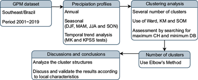
This study aims to assess the application of clustering methods on data from the GPM project to identify homogeneous regions in southeastern Brazil concerning the annual and seasonal precipitation from 2001 to 2019. The WH, KM, and SOM methods are analyzed, and the quality of results are submitted to quantitative measures for further comparison and discussions. This paper is organized as follows: Section 2 presents relevant details about the study area and the GPM data as well as a formal discussion about clustering methods, accuracy measures for clustering assessment, and the study design; Section 3 presents the results and their respective discussions. Section 4 summarizes the findings of this paper.
2. Materials and Methods
2.1 Study Area and Data
The study focuses on southeastern Brazil, located at latitude (25º 18’ 35”S, 14º 13’ 58”S) and longitude (53º 05’ 15”W, 39º 41’ 18”W). The area covers the states of São Paulo (SP), Rio de Janeiro (RJ), Minas Gerais (MG) and Espírito Santo (ES). Figure 1 shows the location and topography of the study area.

Precipitation data for this area were provided by the GPM project from 2001 to 2019. This product estimates daily precipitation at a spatial resolution of 0.1º × 0.1º (Gadelha, 2018). Evaluation of the GPM product over Brazil was done by Rozante et al. (2018) in comparison with rain gauge data. They show that the behavior of maximum precipitation in summer and minimum in winter is well estimated although there is the usual overestimation in summer.
We calculate annual and seasonal accumulated precipitation. The seasons are considered as: summer (December-February; DJF); autumn (March-May; MAM); winter (June-August; JJA); and spring (September-November; SON).
2.2 Clustering Methods
Clustering methods play an important role in exploratory data analysis,
especially in cases where there is little if any knowledge about the data (Jain and Dubes, 1988). Formally, a
clustering comprehends the modelling and application of a function
F: X → Y on a set of
observations
The clustering methods in the literature comprise different approaches to modeling F. Identifying hierarchical relationships, minimizing cluster variability, and performing modeling based on neural networks are some examples of approaches.
Hierarchical methods exploit the relationship structure drawn by the dissimilarity values found between the elements in a dataset. The Ward’s Hierarchical (WH) method (Murtagh and Legendre, 2014) is one of the hierarchical methods, that is defined by the following dissimilarity measure between clusters:
where D(·,·) represents a recursively computed dissimilarity measure over the clusters. This measure corresponds to the Euclidean distance when applied to compare clusters composed by a single element each.
After computing the dissimilarities between clusters throughout D(·,·), a hierarchical organization naturally arises. In turn, it is possible to establish a threshold τ that determines k clusters such that D (G j , G l ) > τ for j ≠ l and j = 1,…,k.
Methods based on minimizing objective cost function define a partition on the dataset such that the variabilities within and between clusters are both minimized and maximized, respectively. Among different methods proposed in the literature following this approach, the K-Means (KM) (Kodinariya and Makwana, 2013) algorithm is highlighted for its simplicity, effectiveness, and robustness. According to this algorithm, the within/between cluster variabilities minimization/maximization are achieved by solving (Webb and Copsey, 2011):
where μ j is the centroid of the cluster G j , for j = 1,…,k.
The optimization problem expressed by Equation 2 is solved iteratively through
the following steps: (i) each observation
Unlike the previous methods, the Self-Organizing Maps (SOM) comprise a data
clustering model based on neural network concepts. Formally, a matrix
L
1
× L
2
of weight vectors w
ij
= [w
ij1
, w
ij2
,…, w
ijn
] denotes a map of neurons. Under these conditions, an observation
where
2.2.1 Clustering Assessment
The use of measures for the assessment of the clustering results is essential to provide a quantitative notion about the quality of the partition obtained and allow comparisons between different results and methods. The Calinski-Harabasz (CH) and Davies-Bouldin (DB) (Debbarma et al., 2019) indices are examples of measures helpful for this purpose.
The quantification performed by the CH measure is based on the variability values from the clusters that define the dataset partition. Assuming that a dataset I is partitioned according to the clusters G 1 ,…, G k , the measure CH is expressed by:
given:
where
The values of CH are in [0, ∞], where higher values imply better clustering results. On the other hand, the CH values tend to decrease as the number of clusters increases. Also, it is worth noting that there is no “acceptable” cut-off value for such measure. Nevertheless, the comparisons should involve results with an equivalent number of clusters and prioritize results with higher CH.
In contrast, the DB index provides an assessment that does not depends on the number of clusters. This measure has been useful in studies related to the analysis of meteorological data (Raju and Kumar, 2007; Pansera et al., 2013) and it is given by:
where
2.2.2 Optimum Number of Clusters
Defining the suitable number of subsets to perform the clustering process may not be a simple task. Distinct approaches in the literature may support this decision. Some examples include the use of Information Criteria concept (Akogul and Erisoglu, 2016), minimizing the error based on Information - Theoretic Standards (Sugar and James, 2003) or even using a heuristic approach based on the explained variance as a function of the number of clusters, also known as Elbow’s Method (Ketchen and Shook, 1996).
Elbow’s Method assumes that the increase in the number of clusters implies a reduction of the accumulated variance inside the clusters. On the other hand, the indiscriminate increase in the number of clusters may not imply significant gains in reducing such variance (Han et al., 2012). This approach has been used in studies related to the determination of homogeneous precipitation regions in different regions of the world, such as Malaysia (Ahmad et al., 2013), India (Akhisha et al., 2018) and Ethiopia (Zhang et al., 2016).
Formally, for a given dataset I partitioned in clusters G j , for j = 1,…, k, the summation of the deviations from the members of each cluster to its centroid may be expressed by:
Consequently, when admitting different values for k
Finally,
2.3 Experiment Design
Figure 2 depicts the experiment design of this study. Firstly, data from the GPM project, expressed in terms of monthly accumulated precipitation, were obtained and limited to the period of interest (2001 to 2019) and study area (Figure 1). Considering this precipitation time series and admitting a significance of 1%, the Mann-Kendall (MK) (Kendall and Gibbons, 1990) and Kwiatkowski-Phillips-Schmidt-Shin (KPSS) (Kwiatkowski et al., 1992) tests were applied to reveal the existence of temporal trend in the data. The precipitation values of each instant in the time series stand for the average value observed in the study area in each season.
Subsequently, the precipitation values were organized into five distinct periods of analysis: annual, which comprises the accumulated precipitation in each year; and seasonal, containing the accumulated precipitation in the seasons of each year in the study period. Specifically, the seasons are: summer (December-February; DJF); autumn (March-May; MAM); winter (June-August; JJA); and spring (September-November; SON).
The KM, WH, and SOM methods (Section 2.2) where applied to the annual and seasonal periods considering the number of clusters varying from 2 to 50. The clustering results (a total of 3 × 49 = 147) are submitted to the CH and DB measures (Section 2.2.1), to determine the most suitable method to identify the precipitation patterns over the study area. An analysis of the optimal number of clusters is then performed using Elbow’s Method (Section 2.2.2). Once the most appropriate method is chosen as well as the optimum number of clusters, the results are discussed considering the topographical and climatic characteristics of the study area.
All the data processing was implemented using the Python 3.8 programming language (van Rossum and Drake, 2011) and the Numpy (Van Der Walt et al., 2011), Scikit Learn (Pedregosa et al., 2011) and GDAL (GDAL/OGR, 2021) libraries.
3. Results and Discussion
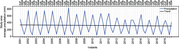
Figure 3 shows the time series of the spatial average precipitation in the study area over the analyzed period, where it is possible to observe a stationary profile. Moreover, both MK (p-value = 0.556) and KPSS (p-value = 0.1) confirm that the precipitation profile has not increased or decreased over the time.
The results demonstrate large spatial variability for the region, as shown in Figure 4. Considering the annual period (Fig. 4(a)), the GPM data shows accumulated precipitation from 800 mm (north of MG state) to 2000 mm (coast of SP state). This spatial pattern agrees with results by Neto (2011), Pampuch et al. (2016), Vasconcellos and Reboita (2021) and Silva et al. (2021).

Fig. 4 Temporal average of precipitation values for the (a) Annual (b) DJF (c) MAM (d) JJA (e) SON regarding the period 2001-2019 using the GPM data.
Considering the seasonal periods (Figs. 4(b) to 4(e)), the patterns agree with precipitation patterns already documented in previous studies (Nunes and Rampazo, 2017; Huffman et al., 2007; Vasconcellos and Reboita, 2021); in summary the highest accumulated precipitation is in summer and it is lowest in winter, with autumn and winter being transition seasons.
In the summer, the highest rainfall values occur on the coast of SP and in the central portion of the southeast sector (about 900 mm) due to the SACZ activity and breeze effects (Vasconcellos and Reboita, 2021). The smallest values are recorded in northern MG state (with 250 mm). The wet summer in the region is characteristic of the SAMS, expressed at upper levels by an anticyclonic circulation over Bolivia and a trough near the coast of northeastern Brazil. High pressure systems and an anticyclonic circulations over the sub-tropical Pacific and Atlantic oceans, a low pressure over northern Argentina (Chaco), SACZ, and the South American Low-Level Jet east of the Andes are observed at low levels (Marengo et al., 2010). All these circulation patterns are responsible for more than 60% of the precipitation that occurs in this season (Vasconcellos and Reboita, 2021).
The transition between summer and winter (Fig. 4(c)) has characteristics of both seasons and shows precipitation values from 200 to 600 mm. This season is characterized by a reduction in solar heating and convection, weakening of the trade winds and actuation of the SASH (Vasconcellos and Reboita, 2021). Thus, it is possible to notice a reduction in rainfall compared to the previous season (summer), but not intense as in the winter.
It is evident from the GPM data that the lowest precipitation values (about 0 and 300 mm) are observed in June, July and August. Neto (2011) showed that in the period 1961-2011 less than 5% of the accumulated annual precipitation occurred in winter. In this situation, the SASH is displaced westward, affecting southeastern Brazil and preventing the equatorward advance of frontal systems (Vasconcellos and Reboita, 2021; Silva et al., 2014).
The spring season shares similarities with autumn and shows a rainfall increase compared to winter. This increase in precipitation occurs due to the increase in heating and the establishment of the SAMS atmospheric systems (Marengo et al., 2010; Vasconcellos and Reboita, 2021). The average precipitation ranges from 200 to 400 mm.
The performance of the KM, WH, and SOM methods for clustering precipitation data with a different number of clusters (2 to 50) was then assessed through the CH and DB measures (see experiment design in Fig. 2) and distinct periods of analysis (i.e., annual and seasonal). Figure 5 depicts this assessment, where the KM method shows better results compared to the WH and SOM methods, as it often displays high CH and low DB values independently of the number of clusters. The dashed lines indicate the central tendency in which each method, regarding the CH and DB measures, behaves as a function of the number of clusters. Based on this tendency profile, the KM method always provides higher CH values and lower DB values, implying a better performance than the WH and SOM methods regardless of the period considered (annual or seasonal).

Fig. 5 Clustering assessment based on CH and DB indexes for distinct periods of analysis and number of clusters.
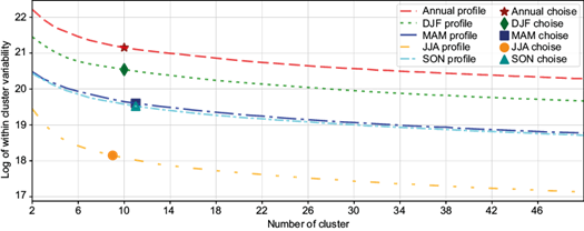
Once the KM method is identified as the most suitable to cluster precipitation data, the optimal number of clusters was analyzed using the Elbow’s Method. Figure 6 illustrates the relation between log Q(k) to k from 2 to 50. The values for k that maximize L(k; 2, 50) for each period are highlighted as symbols in Figure 6, indicating 10 clusters for the annual and DJF periods, 11 clusters for the MAM and SON periods and 9 clusters for JJA.
Based on the optimal number of clusters for each period, Figure 7 maps the regions with distinct precipitation patterns over the study area. Figures 8, 9, 10, 11 and 12 shows the annual/seasonal averages extracted from each region, allowing to infer the rainfall regimes of the considered periods and respective partitioning.

Fig. 7 Clustering results for each analyzed periods using the KM method and optimal number of clusters.

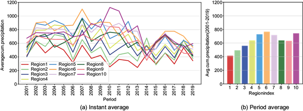


The annual period, clustered into 10 regions, reinforces the consistency of the results, which agree with homogeneous precipitation regions compared to climatology (Figure 4). The highest accumulated precipitation (1600 mm) is found on the coast of SP (region 9), decreasing to the north towards region 1, where the smallest precipitation amount is observed (740 mm). The annual variability is similar in all regions. Note that a decrease in precipitation in all regions occurred in 2014, associated with the well-known drought event observed that year in the study region (Coelho et al., 2016; Otto et al., 2015; Nobre et al., 2016).
Precipitation during summer (DJF) clustered into 10 regions, indicates the highest rainfall, about 750 mm (region 6) in the northern portions of SP and the southwest of MG states. Precipitation decreases in the center of SP and reaches the lowest values in the north of MG, about 400 mm (region 1). Summer corresponds to the largest seasonal precipitation accumulated in all regions, due to the SAMS as mentioned above. Nevertheless, summer precipitation indicates a remarkable interannual variability between clusters.
Precipitation during autumn (MAM), clustered into 11 regions, clearly separate regions with high (450 mm) and low (190 mm) accumulated precipitation, corresponding to the coast of SP (region 10) and north of MG (region 1), respectively. There is a reduction in accumulated precipitation compared to summer. Considering the annual variability in MAM, the pattern is similar for all regions, except in 2011 in region 7, where the largest accumulated precipitation of the entire series was recorded in this season.
Precipitation during winter (JJA), clustered into 9 regions, shows that the north of MG state comprises a vast region, while the SP state is divided into several regions. The largest precipitation is observed in region 9 (255 mm) and the smallest in region 1 (20 mm). The large amounts of precipitation in the south and southeast portions are associated with cold fronts that may reach the region and the SASH area. Winter is the season with both less accumulated precipitation and similar annual variability in all clusters.
Precipitation during the spring (SON) season, clustered into 11 regions, mark separations at the north of MG, the central portion of SP, and the coastal zone of RJ. The difference in accumulated rainfall between regions is not as evident as in other seasons, and the values range from 280 mm and 400 mm. The accumulated precipitation increases during spring as the atmospheric systems characteristic of the SAMS become established. The annual variability in spring is similar for all clusters except in 2015, where the dry period does not occur with the same intensity in all regions.
4. Conclusions
This study presents an analysis of the distribution of precipitation patterns in southeastern Brazil using different clustering methods applied to data from the GPM project.
The results obtained indicate that the GPM data reveal a precipitation distribution consistent with the seasonal characteristics already discussed by Neto (2011), Pampuch et al. (2016), Vasconcellos and Reboita (2021) and Silva et al. (2021), as Figure 4 demonstrates: (i) an increase in precipitation in DJF; (ii) a gradual decrease in precipitation in MAM; (iii) the lowest precipitation values occur in JJA; and (iv) in SON a gradual increase in SON.
The annual analysis indicates that the coastal regions of São Paulo and Rio de Janeiro concentrate the highest precipitation in the study area. The precipitation volume decreases significantly towards the north and northeast regions.
According to the CH and DB measures applied to analyze the performance of the different clustering methods, the KM algorithm was the most suitable for identifying the regions of distinct precipitation patterns. The Elbow’s Method was then applied to determine the optimum number of regions that partitions the study area in each period (i.e., annual and seasonals).
Based on these analyses the following can be inferred:
Seasonality - seasonal and annual distributions have different impacts on the analysis of rainfall patterns in the study area, as they can be influenced by various factors such as convergence zones, droughts, longer duration of the rainy season, fires and others. The highest precipitation is observed in summer and spring and the lowest in winter.
Clustering method - the KM algorithm is identified as a suitable clustering method in the domain considered, becoming more refined through the Elbow’s Method. A remarkable similarity is found in the precipitation regime, both for the annual and the seasonal periods.
Finally, no prior studies have used this combined methodology for the southeastern region of Brazil, since Pampuch et al. (2016) used Ward’s Hierarchical clustering and Singular Value Decomposition, and Machado (2014) used K Means. Consequently, analyses with similar methodology should be carried out in future studies to identify subgroups within the presented clustering and obtain more information about the precipitation regime in southeastern Brazil.

