


 nueva página del texto (beta)
 Inglés (pdf)
 Artículo en XML
 Referencias del artículo
 Enviar artículo por email
 Citado por SciELO
  Similares en
SciELO
Similares en
SciELO 
 Permalink
1. Introduction
In 2015, the World Health Organization (WHO) recognized ambient air pollutant exposure and its effects on human health as a public health priority requiring further study (WHA68, 2015). The rapid expansion of urban areas worldwide has increased the number of individuals exposed to pollutant concentrations above the upper limits recommended by the WHO (Riojas-Rodríguez et al., 2016). For instance, the Mexico City Metropolitan Area (MCMA) is the third-largest metropolitan area of the member states of the Organization for Economic Cooperation and Development (OECD) and is considered one of three megacities in Latin America (OECD, 2016). Historically, this area has registered high rates of air pollution (INE-SEMARNAT, 2011), posing a constant risk to the health of its nearly 21 million inhabitants (INEGI, 2015).
Epidemiological studies have shown that chronic exposure to ambient PM2.5 and NO2 is associated with health outcomes including increased mortality (Beelen et al., 2014), cardiovascular disease (Dockery, 2001; Hoek et al., 2013), lung cancer (Pope et al., 2002; Chen et al., 2008; Hamra et al., 2014), cardiopulmonary conditions (Krewski et al., 2009) and diabetes (Li et al., 2014). These studies have used a variety of methods to estimate air pollutant exposure and have developed deterministic and/or probabilistic models as the cornerstone of their analyses. In Mexico, the majority of epidemiological studies on the health effects of air pollutants have estimated pollutant exposure using proximity methods, such as those based on data from the nearest air quality monitor (Rojas-Martinez et al., 2007; Barraza-Villarreal et al., 2008; Escamilla-Nuñez et al., 2008; Hernández-Cadena et al., 2009), averages by city or municipality (Téllez-Rojo et al., 2000; Carbajal-Arroyo et al., 2011), or Inverse Distance Weighting (IDW) interpolation (Riojas-Rodríguez et al., 2014; Trejo-González et al., 2019). One disadvantage of these approaches is their failure to capture the spatial variability of exposures caused by local pollution sources, urban topography and local meteorological factors (Jerrett et al., 2005), which leads to considerable uncertainty regarding accurate exposure estimation. To the best of our knowledge, the available literature offers few epidemiological studies which have employed more sophisticated, high-resolution methods (e.g., based on satellite data) for estimating exposure to ambient air pollutants in the Mexican population (Rosa et al., 2017; Gutiérrez-Ávila et al., 2018; Téllez-Rojo et al., 2020). Furthermore, previous studies have noted that human exposure to air pollutants can differ between individuals due to variable factors such as time spent outdoors and mobility patterns, thereby introducing bias into individual-level exposure estimates in epidemiological analyses (Setton et al., 2011; Nyhan et al., 2019; Yu et al., 2020).
To offset these limitations, our study has geocoded the home and work addresses of the study population and fitted generalized additive models (GAMs), which predict PM2.5 and NO2 concentrations at both locations. The principal advantage of the GAMs is their use of semiparametric methods to model non-linear functions through penalized splines (Yanosky et al., 2008).
This study represents a refinement of exposure models previously developed and applied in the MCMA (Just et al., 2015; Rivera-González et al., 2015; Son et al., 2018). In order to craft a feasible model adaptable to the limited information available in developing countries, we used the highest-quality and largest amount of secondary source data available on air pollutant predictors in Mexico. This study therefore provides a novel methodological tool to be used in the Mexican Teachers’ Cohort (MTC) study, as well as for subsequent epidemiological studies which seek to assess the effects of PM2.5 and NO2 exposures on health. Our aim was to determine the level of monthly exposure to outdoor PM2.5 and NO2 of approximately 16 500 MTC participants living and working in the MCMA between 2004 and 2019.
2. Material and methods
We developed spatiotemporal prediction models for PM2.5 and NO2 using the pollutant concentrations at monitoring locations as the dependent variable, and meteorological and geographic variables, as well as other pollutants, as predictors. For statistical modeling, geostatistical modeling, geoprocessing and spatial analysis, we used R software version 3.5.3 (R Core Team, 2019).
2.1 Study population and geocoding
This study is nested within a larger study known as the MTC, an ongoing prospective observational study established in 2006-2008 that includes 115 314 female public-school teachers from 12 Mexican states, with a median age at enrollment of 44 years. A detailed description of the full cohort has been published elsewhere (Lajous et al., 2015). In brief, recruitment was divided into two phases: the first (2006) took place in two states (Jalisco and Veracruz, n = 27 979), and the second (2008) incorporated 10 additional states (Baja California, Chiapas, Mexico City [CdMx], Durango, Guanajuato, Hidalgo, Mexico State [EdoMex], Nuevo León, Sonora and Yucatán, n = 87 335). Participants completed a reference questionnaire with sociodemographic characteristics (including home address [HA] and work address [WA]), reproductive history, diet, lifestyle and health status. Follow-up takes place every 3-4 years to obtain information on any disease diagnoses and update participant risk factor profiles. The first follow-up cycle (2011-2013) obtained a response rate of 83%, and the second cycle (2014-2020, ongoing) of 61%.
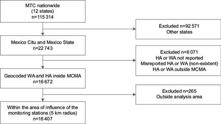
For the present study, we selected a subsample of the MTC which excluded participants with the following characteristics: (1) from states other than CdMx or EdoMex (n = 92 571), (2) without a valid HA or WA on file (n = 6071), or (3) with an HA or WA unable to be geocoded inside the area of influence of the MCMA environmental monitoring network (n = 265, methods described below). The analysis included a total study population of n = 16 407 MTC participants.
The original MCMA is composed of 16 municipalities of CdMx, 59 of EdoMex and one of Hidalgo. We did not include the entire MCMA due to the low/under-representation of pollutant measurements at locations far from monitoring stations, which do not achieve full coverage of the area (Fig. 1). Based on this determination, we drew the boundaries of the analysis area using the extreme coordinate position of a 5 km radius around each of the most peripheral monitoring stations. Within these boundaries, we defined a grid composed of 1 × 1 km cells (in gray, Fig. 1).

Fig. 1 Area of analysis and geocoded addresses. (a) Location of work addresses at baseline (2008) and first follow-up cycle (2011-2013). (b) Location of home addresses and number of teachers per zip code.
We geocoded the HA and WA of each participant within the study population. For HA, we geocoded zip codes (ZC) as reported at baseline. Based on the Mexican Postal Service (SEPOMEX) criteria for valid ZCs, we selected only those containing five digits and verified that the first two corresponded to the codes of home municipalities also reported by teachers. Finally, we used the geographical layer of SEPOMEX’s ZCs (Gobierno de México, n.d.) to assign the coordinates of the ZC’s centroid to each HA. Since information on HA changes was unavailable for before and after the baseline, we assumed that HA were constant throughout the follow-up period. To geocode WAs at baseline and follow-ups, we used the workplace codes provided by the National Teaching Career Program. The geographic coordinates (longitude and latitude) were matched from the National School Information System (SEP, n.d.).
2.2 Meteorological and air pollutant data
We obtained databases of hourly pollutant measurements (PM10, PM2.5, SO2, NO2 and O3) and relevant meteorological variables (relative humidity, temperature and wind speed) for all monitoring sites within the area of interest from 1:00 LT on January 1, 2004 to 12:00 LT on July 31, 2019. Datasets were provided by the monitoring network of Mexico City’s Environmental Ministry and remain permanently available for public consultation on the official websites (Gobierno de la Ciudad de México, n.d.).
We calculated daily and monthly estimators (averages) for each pollutant and meteorological variable at each monitoring station where a minimum of 75% of the required observations were available (18 h and 23 days, respectively). Otherwise, we recorded data as missing and those observations were not part of the complete case analysis (more details in the statistical analysis section). Seasons, used as a categorical variable, were defined as follows: the cold-dry season from November to February, the hot-dry season from March to May, and the rainy season from June to October.
2.3 Geographic data and other covariables
Geographic profiles of the monitoring sites were characterized using a geographic information system (GIS). We created a geographical layer of the air quality monitoring stations in place from 2004 to 2019 in the study area, based on coordinates provided by the National Air Quality Information System (SINAICA) (INECC, n.d.). The altitude variable was provided by SINAICA in meters above sea level (masl) and categorized into tertiles as follows: low as ≤ 2300 masl, medium as ≥ 2301 and ≤ 2500 masl, and high as ≥ 2501 masl. The vehicle motorization index (number of motorized vehicles per 1000 inhabitants) was calculated annually at the municipal level, based on population projections from the National Population Council (Gobierno de México, n.d.) and historical databases of registered motor vehicles in circulation (automobiles, passenger buses, cargo trucks and motorcycles), according to the Mexican National Institute of Statistics, Geography and Informatics (INEGI, n.d.). This variable was categorized into tertiles as follows: low as ≤ 222 vehicles per 1000 inhabitants, medium as ≥ 223 and ≤ 487 vehicles per 1000 inhabitants, and high as ≥ 488 vehicles per 1000 inhabitants.
2.4 Statistical analysis
2.4.1 Generalized additive models (GAMs) and validation
To determine the contribution of each predictor to PM2.5 and NO2 variability at monitoring stations between 2004 and 2019, we fitted two independent GAMs (Eq. [1])
where f j (.) are smooth functions, Y is the vector of outcomes and the X j are the vectors of covariates. We performed a complete case analysis for each model, using monthly PM2.5 or NO2 concentrations per monitoring site as the dependent variable. Due to its skewed distribution, the vector PM2.5 was log-transformed. Models only included covariables expected a priori to exert a physical influence on the PM2.5 and NO2 levels. Predictors introduced in the adjusted models were the group of other pollutants, the meteorological variables and the geographical variables. To account for the correlation between pollutants, we included them with interaction terms. To ensure a parsimonious model specification, we tested the contribution of each term by eliminating it in the model and retained only those which improved predictive accuracy and showed statistical significance (p < 0.05). Model comparison and selection were performed according to deviance explained (DE), Akaike information criterion and root mean square error (RMSE). To test the goodness of fit, we performed a residual diagnosis allowing us to verify normality and the absence of any overdispersion patterns. Finally, we performed stepwise selection to test and select the number of base functions needed to achieve a smooth curve which would maximize our data fit and reduce RMSE.
To test the GAMs for possible overfitting and evaluate their predictive accuracy, we carried out a 10-fold cross-validation and determined the predictive accuracy of each model based on its cross-validation root mean square error (CV-RMSE).
2.4.2 Model predictions and geostatistical conditional simulation
We used the GAM coefficients to predict the monthly concentrations of PM2.5 and NO2 in each 1 × 1 km grid cell from January 2004 to July 2019. For each grid cell and for each month of the study period, we carried out 3000 simulation replicates using the Geostatistical Conditional Simulation (GCS) method (ESRI, n.d.) with the aim to obtain the mean value of the predictor variables: PM10, O3, SO2, NO2, wind speed, relative humidity and temperature in each cell. As part of the GCS, we fitted Gaussian and exponential variograms with and without the nugget effect to empirical semivariograms in order to characterize the spatial structures at unmeasured locations (Eq. [2]). To this end, we used the Cholesky decomposition of covariance matrix (Chilès and Delfiner, 2012):
where the degree of spatial dependence among the values of attribute Z in two different locations or points in space was semivariance γ(h), and the distance between the points was lag h.
To account for error ϵ ij in the GAMs caused by the spatial correlation of the observations, we carried out the same simulation procedure with the residuals before adding them to the predicted values for each grid cell.
2.5 Assigning of cohort participant exposures
To maximize the precision of exposure estimates, we accounted for the intra-city mobility of study participants by assigning predicted monthly values for PM2.5 and NO2 for each month during the study period to the grid cell where the HA and WA of each teacher were located. With the assumption that mobility-based estimates (HWA weig ) were closer to actual exposure (individual monitoring), HA and WA exposures were weighted according to the number of hours spent at each address, assuming the average length of the Mexican workday (8 h) (Eq. [3]).
To assess the relevance of mobility to our study, we compared HA and WA exposures by calculating the difference between HA-HWA weig . The null hypothesis (a difference of zero) was proved using a mixed-effects model, where the teacher was the grouping variable.
3. Results
3.1 Study population and geocoding
The national-level MTC included 115 314 total participants, of which 22 743 lived either in the CdMx or EdoMex. From this subsample, we were able to geocode HA and WA within the MCMA of 73% (n = 16 672). In terms of HAs, the median of teachers per ZC was 23, with a range of one to 175 (Fig. 1). The areas of these ZCs ranged from 0.005 to 17.003 km2. Therefore, the final study population included 16 407 MTC participants who lived and worked in the area of analysis (Fig. 2), covering (totally or partially) 72 municipalities in the CdMx or EdoMex.
3.2 Descriptive statistics
Monthly averages of PM2.5, NO2 and their predictor variables at the monitoring site level are summarized in Table I. During the 2004-2019 period, a maximum of 11 and 17 monitoring stations for PM2.5 and NO2, respectively, provided data on all variables required to adjust the GAMs. The geometric mean and SD of monthly PM2.5 concentrations were 3.18 and 0.27 µg m-3, respectively, and the mean and SD of monthly NO2 concentrations were 28.34 and 8.59 ppb, respectively. Over the study period, the mean ambient temperature was around 17 ºC (range 5, 23), wind speed averaged 1.85 m/s (range 0.49, 4.95) and average humidity was 55% (range 28, 88). The lowest concentrations of both pollutants were registered during the rainy season, and the highest during the cold-dry season. PM2.5 concentrations were greatest at the lowest altitudes.
Table I Descriptive statistics for final GAM predictor variables, and bias and precision statistics from cross-validation.
| Variable | Time- varying | Model | |
| PM2.5 mean (SD) n = 779 | NO2 mean (SD) n = 1298 | ||
| Monitoring stations included 2004-2019 period (min-max) | 3-11 | 6-17 | |
| PM2.5 (µg m-3) | Yes | 25.05 (6.90) | --- |
| NO2 (ppb) | Yes | 29.83 (8.02) | 28.34 (8.59) |
| O3 (ppb) | Yes | --- | 27.95 (7.14) |
| PM10 (µg m-3) | Yes | 49.67 (17.15) | 50.41 (18.66) |
| SO2 (ppb) | Yes | --- | 6.93 (4.23) |
| Temperature (ºC) | Yes | --- | 16.71 (2.18) |
| Wind speed (m/sec) | Yes | 1.90 (0.50) | 1.81 (0.47) |
| Relative humidity (%) | Yes | 52.54 (11.40) | --- |
| Season a Rainy (ref) Cold-dry Hot-dry | No | 19.73 (3.90) 29.12 (6.30) 27.90 (5.88) |
23.42 (6.35) 33.13 (8.62) 28.83 (7.39) |
| Motorization index (no. vehicles/1,000 ha) a High (ref) Medium Low | Yes | --- --- --- |
27.60 (7.47) 29.35 (8.77) 27.52 (9.68) |
| Altitude (m) a High (ref) Medium Low | Yes | 19.80 (4.53) 24.96 (6.10) 26.36 (7.20) |
--- --- --- |
| Year a 2004 (ref) 2005 2006 2007 2008 2009 2010 2011 2012 2013 2014 2015 2016 2017 2018 2019 |
28.32 (5.75) 29.26 (9.94) 29.09 (6.41) 28.16 (4.92) 26.80 (7.10) 24.07 (5.88) 23.63 (8.01) 24.87 (7.95) 23.39 (4.49) 25.33 (7.47) 23.22 (6.14) 24.96 (5.75) 24.39 (6.97) 24.66 (7.75) 24.05 (5.91) 24.15 (6.37) |
33.97 (7.15) 34.02 (8.86) 33.14 (7.22) 33.04 (7.64) 31.73 (7.17) 30.70 (7.25) 32.14 (8.49) 28.06 (8.88) 27.78 (8.77) 25.98 (7.96) 26.06 (7.47) 23.92 (7.21) 24.80 (7.66) 25.74 (8.25) 25.72 (7.30) 22.20 (6.67) |
|
| Statistics | Model | ||
| PM2.5 | NO2 | ||
| DE | 87.3% | 74.4% | |
| RMSE | 0.100 | 4.406 | |
| CV-RMSE | 0.102 | 4.497 | |
aVariable included is categorical; however, for descriptive purposes, mean (SD) is presented for the dependent variable in each category.
DE: deviance explained; RMSE: root mean square error; CV: cross-validation.
3.3 Generalized additive model for PM 2.5 and predicted values
The PM2.5 model predictors were altitude, relative humidity, wind speed, season and year, in addition to the pollutants PM10 and NO2. Only PM10, relative humidity and wind speed were included as continuous variables with smoothing functions, using penalized splines of up to seven degrees of freedom (Fig. 3).
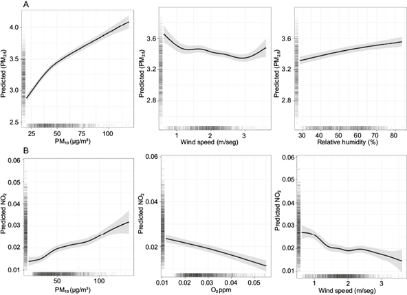
Fig. 3 Smooth plots from the final models showing non-linear effects of selected predictors and associated predicted PM2.5 (uptrend) and NO2 (downtrend) concentrations. CI is set at two standard errors above and below the mean.
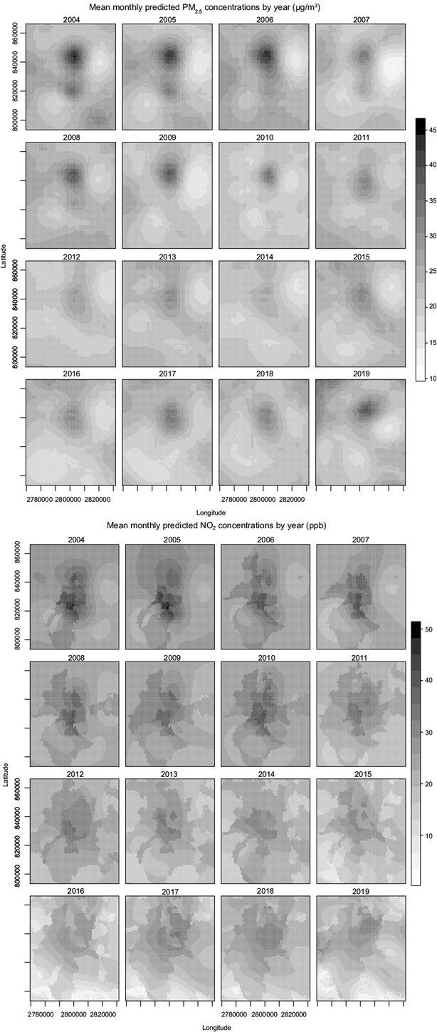
The maps in Figure 4 illustrate the average spatial distribution of the monthly PM2.5 levels predicted by the model per year on the surface of the area of analysis (the grid). In general, predicted levels were higher further north within the MCMA and trended downwards until 2014. The 2019 map considers only measurements until July; therefore, the rainy season, which yielded the lowest PM2.5 levels (see Table I), was underrepresented. The percentage of deviance explained by the model was high (DE = 87.3%) for the 2004-2019 period (Table I). The RMSE in the sample indicated high predictive accuracy with a low level of error (RMSE = 0.100), and showed no overfitting of data, as determined by its proximity to the cross-validation error (CV-RMSE = 0.102).
3.4 Generalized additive model for NO 2 and predicted values
The NO2 model predictors were the vehicle motorization index, wind speed, temperature, season and year, in addition to the pollutants PM10, O3 and SO2. Only PM10, O3 and wind speed were included as continuous variables with smoothing functions using penalized splines of up to seven degrees of freedom, since the other continuous variables showed a linear relationship with the dependent variable (Fig. 3). The maps in Figure 4 show the model predictions of average spatial distribution of monthly levels of NO2 within the study area per year. In general, the predicted levels of NO2 were highest in the center of the MCMA and trended downwards until 2016, with a mean of 16.87 ppb (SD = 7.77) within the study area. As with PM2.5, only measurements until July 2019 were considered. The percentage of deviance explained by the model was intermediate (DE = 74.4%) for the 2004-2019 period (Table I). The RMSE in the sample indicated high predictive accuracy with a low level of error (RMSE = 4.406) and showed no overfitting of data, as determined by its proximity to the cross-validation error (CV-RMSE = 4.497).
3.5. Exposure assignment adjusted for mobility
All teachers reported a HA different from their WA, which strengthens the case for considering mobility when estimating air pollutant exposure. For the time period and population analyzed, the ranges of differences in estimated exposure at the homes and workplaces of participants were 0-6.01 µg m-3 for PM2.5 and 0-14.76 ppb for NO2. Only 0.11% (n = 1799) of teachers changed WAs between the first and second follow-up cycles. On average, they traveled 6.285 km (SD = 6.216) between their homes and their workplaces (min: 0.0098 km, Q1: 1.846 km, Q2: 4.282 km, Q3: 8.746 km, max: 56.155 km).
We obtained 187 weighted monthly averages of PM2.5 and 187 of NO2 assigned to each teacher as a proxy for long-term exposure. Figure 5 illustrates the annual distribution and principal statistics for the weighted monthly averages (HWA weig ) assigned to the 16 407 MTC participants during the 2004-2019 period. For both pollutants, we determined the expected exposure variability attributable to the spatial distribution of pollutants and the location of HAs and WAs within the study area. On average, for the population and period analyzed, weighted exposures were 24.38 µg m-3 (SD = 6.78) to PM2.5 and 28.21 ppb (SD = 8.00) to NO2.

Fig. 5 (b, d) Violin plot and descriptive statistics for assignment of monthly PM2.5 (B and D) and NO2. (a, c) weighted exposures () by year. First, second and third quartiles estimated for n = 16 407 teachers.
Average exposures to both pollutants were lower at HAs than at HWA weig (PM2.5: HA 24.37 µg m-3, HWA weig 24.39 µg m-3; NO2: HA 28.15 ppb, HWA weig 28.21 ppb). Average differences were -0.016 (range -2.00-1.91) for PM2.5 and -0.063 (range -4.92-4.60) for NO2. In both cases, the differences between HA and HWA weig did not equal zero and were statistically significant (p < 0.0001).
4. Discussion
The models developed in our study provide a useful method for predicting monthly exposure to outdoor PM2.5 and NO2 at any location within large areas throughout the MCMA, with high spatial (1 × 1 km) and temporal (16 years: 2004-2019) resolution. These models performed well and delivered high predictive accuracy, with cross-validation errors slightly higher than those of the models (CV-RMSE = 0.102 for PM2.5 and CV-RMSE = 4.497 for NO2). A large difference between these values would have suggested that GAMs overfit the data, as performance would have been lower in data not included in the adjustment during cross-validation. Because of their high resolution, these models satisfy the permanent need of epidemiological studies to predict and assign exposures to ambient air pollutants in numerous MCMA locations with a high degree of precision. Furthermore, they cover a long time period (16 years) on a small temporal scale (monthly), allowing the assessment of effects of medium- and long-term exposures.
To our knowledge, only three published studies have proposed models for determining exposure to ambient air pollutants in Mexico (Just et al., 2015; Rivera-González et al., 2015; Son et al., 2018), of which all focus on Mexico City and/or the MCMA. Rivera-González et al. (2015) provide a comparison of four basic methods based on proximity and interpolation for all criteria pollutants. The principal limitation of several of these approaches is that they do not capture the spatial variability of exposure (Jerrett et al., 2005). Our study overcomes this limitation by using high spatial resolution, which captures much greater variability. Son et al. (2018) proposed a mixed-effects regression model based on land use for all criteria pollutants. Although this study follows the traditional assumption of a linear relationship between predictors and the dependent variable, it is innovative in that it explores the statistical model-fitting techniques of least absolute shrinkage and selection operator (LASSO) method, in addition to analyzing various spatiotemporal scales (hourly, daily, monthly, semi-annual and annual). Instead of this model, our study proposes GAMs, which maximize the quality of dependent variable prediction by accounting for its non-linear relationship with the predictors, and incorporate smoothed (non-parametric) terms using penalized splines. However, we explored a monthly exposure scale for only two criteria pollutants. Finally, Just et al. (2015) developed a more sophisticated mixed-effects regression model, including satellite-based aerosol optical depth measurements as primary PM2.5 predictor, over a period of 10 years. While innovative, this method is limited in that it cannot be applied where little or no PM2.5 monitoring data exist for validation, and also because no satellite measurements can be taken on cloudy days (Paciorek and Liu, 2009; Bravo et al., 2012). We overcame this first limitation, an obstacle faced by many developing countries, by using information on predictors from secondary sources which are easily accessed and interpreted, and are permanently monitored. Furthermore, we covered a longer time span (16 years) and also modeled NO2 exposure. Despite important distinctions from previous studies, we obtained largely similar results; predicted spatial patterns for PM2.5 were comparable and, on average, predicted concentrations for both pollutants (PM2.5 and NO2) were only slightly lower.
The results of our analyses demonstrate the relevance of using meteorological variables and other pollutants as primary PM2.5 and NO2 predictors. This could indicate the feasibility of generating highly predictive models using only secondary monitoring data from local networks. Our study therefore confirms that, despite limited availability of information, it is possible to design feasible methods for predicting outdoor exposure to air pollutants, including for other pollutants (such as PM10) when no data is available on PM2.5, as is the case in multiple cities within developing countries. In terms of spatiotemporal prediction of PM10, we expect to observe predictive accuracy as high as that of PM2.5, since in urban areas both fractions of PM have similar potential sources, though in different proportions (Karagulian et al., 2015). Furthermore, geographical predictors are a key consideration given the nature of the contaminants of interest and the geographical characteristics of the study area. In the two models we developed, the geographical predictors showed smaller coefficients than the other predictors. In addition to altitude and the vehicle motorization index, we generated and tested other geographical variables. The linear meters of different types of avenues in buffers of 100-, 300- and 500-m diameters around the monitoring stations did not prove to be significant and therefore were not included in the final models. We tested the UV-B radiation variable and found a significant relationship with NO2; however, it was excluded from the final model due to insufficient monitoring sites in the study area (only 0-6 stations during the 2004-2019 period) which did not allow a semivariographic analysis, causing an increase of 0.583 units of CV-RMSE in the NO2 model (CV-RMSE including UV-B = 3.914).
A recent study which analyzed and compared the home-work mobility patterns of approximately 400 000 individuals, affirmed that ignoring mobility causes erroneous classification when estimating health effects (Nyhan et al., 2019). The principal strength of our study was in considering home-work mobility to estimate PM2.5 and NO2 exposures. Given the findings of Nyhan et al. (2019), we expect that this consideration will help reduce measurement errors that could lead to null association measurements in subsequent epidemiological studies. Another strength of our study was the method used to ascertain the spatial distribution of predictor variables at unmeasured sites. Although no existing method can offer an exact estimate of an unknown reality, GCS considers the dispersion of the phenomenon analyzed and allows the obtention of one among the possible spatial of a random function (surface). The simulated variables thus present the same variability and correlation characteristics as the observed data (measured according to their mean, variance and semivariogram) (Goovaerts, 1997; Deutsch and Journel, 1998). Other potential methods considered included IDW interpolation or kriging; however, despite their extensive application in earth and environmental sciences, these provide only a smooth image of reality, whereas GCS assumptions include seasonality and a normal data distribution (Goovaerts, 1997; Deutsch and Journel, 1998).
We are aware that inherent precision and measurement errors exist in predictive models such as the one we developed, which depend not only on mobility but also on the residential history of participants and precise geocoding of addresses. Prior studies have suggested that the geocoding technique can influence health effect estimates when using fine-scale exposure models (Jacquemin et al., 2013). Therefore, we recognize three sources of error. First, we assumed that the HAs of cohort participants were permanent throughout follow-ups, supported by a previous study by Pimienta-Lastra and Toscana-Aparicio (2019) that registered low inter-municipal migration within the MCMA (4.8%) from 2010 to 2015 (Pimienta-Lastra and Toscana-Aparicio, 2019), thereby suggesting that our study population was similarly unlikely to change addresses. Second, we assessed HAs by geocoding the centroids of their corresponding ZCs as opposed to using exact HA coordinates, and ZC areas varied widely (0.005-17.003 km2) among participants. Previous studies have documented that estimating air pollution exposure by certain zones such as zip codes implies greater uncertainty, as compared to estimation by exact home addresses (Kinnee et al., 2020); however, since home addresses were not available, we used zip code centroids as a proxy of participant residence. Finally, we assumed that the long-term outdoor exposure levels determined were also a reasonable representation of interior and microenvironment exposure.
The models developed were subject to various limitations. First, determination of the study area and population was restricted by the quality of secondary available data (the geographical layer of ZCs) to geocode the HAs of the MTC participants. Although the cohort was extended across 12 Mexican states, we were able to partially include only two of them in this study. Second, given the suboptimal quality of available data, we did not include the characterization of pollution sources attributable to land use and vehicular traffic emissions. Nonetheless, as a proxy for the latter, we used a vehicle motorization index created with official data on registered vehicles at the municipal level. This data was used under the assumption that it would stay constant within each municipality, and inter-municipal mobility was not considered. The vehicle motorization index variable proved significant in the NO2 model, but not the PM2.5 model, which is consistent with our theoretical framework given that NO2 is primarily generated by fuel combustion in vehicles. The result of including aggregated variables to the models may have been a misclassification of predictions’ spatial variability, as a result of the dilution of all possible values within each aggregated area. Finally, another important limitation to consider was the lack of monitoring data, which limits the type of statistical and spatial analyses possible. Air pollution models require datasets with sufficient data for training models and validation, therefore less available data limits the statistical techniques than can be applied to achieve prime model performance or cross-validation.
5. Conclusions
In conclusion, it is crucial for environmental epidemiology to apply methods for the estimation of ambient air pollutant exposure that can overcome limited data availability, which is a particularly relevant factor in developing countries. Our results suggest that the model presented herein offers a promising alternative to be used in epidemiological studies for predicting PM2.5 and NO2 exposure with high spatiotemporal resolution within the MCMA in the 2004-2019 period. Beyond the MCMA context, these models can be replicated in other cities using similar information sources. Our results highlight the importance of developing pollutant exposure models with high predictive accuracy based on available secondary data from official sources. Further research should focus on expanding these models to other Mexican cities.

