


 nueva página del texto (beta)
 Inglés (pdf)
 Artículo en XML
 Referencias del artículo
 Enviar artículo por email
 Citado por SciELO
  Similares en
SciELO
Similares en
SciELO 
 Permalink
1. Introduction
Precipitation is a vital parameter of the Earth’s weather system (Partal, 2018); it synthesizes the behavior of the climate in a region (Pabón-Caicedo et al., 2001) and is a significant source of information for meteorological and hydrological studies (Navarro de León et al., 2005; Guijarro, 2014; Li et al., 2020; Morales et al., 2021).
Climatological data with unreliable or missing values is an important area of research, and there are multiple methods available to fill in missing data (Suhaila et al., 2008; Firat et al., 2012; Kang, 2013; Azman et al., 2015; Kanda et al., 2018; Morales et al., 2019;) and evaluate data quality. Missing data frequently occur due to various problems, including issues with the measuring devices, measurement errors, absence or replacement of the observer, loss of records, relocation of stations, urbanization of the area, and natural hazards (Suhaila et al., 2008). Meanwhile, the loss of homogeneity in a time series of meteorological observations is a consequence of changes in the methodology used, the conditions around the station, and the lack of reliability of the measurement tool (Firat et al., 2012; Guijarro, 2014; Kamaruzaman et al., 2017).
Numerous studies have explored various methods for the imputation of missing values of climatological and hydrological variables, which include distance weighting techniques (Radi et al., 2015), linear regression (Aieb et al., 2019), artificial neural networks (Norazizi and Deni, 2019), and geostatistical techniques (Wagner et al., 2012). For example, Norazizi and Deni (2019) compared the performance of an artificial neural network, bootstrapping, expectation maximization, and multivariate imputation by chained equations (MICE) methods. Their outcomes showed that the artificial neural network had the best performance, but this method involves complex mathematical formulation that requires intensive calculations with high computational cost (Campozano et al., 2014; Miró et al., 2017). When Kriging and Co-Kriging techniques were compared with MICE by Carvalho et al. (2017), MICE provided better estimates of daily precipitation values. Wagner et al. (2012) compared the performance of the spatial interpolation approach applied to precipitation via seven methods, including the deterministic Thiessen polygon method, statistical and geostatistical approaches, where regression-based methods performed best.
Several methods have also been proposed to test the homogeneity of climatological variables, including precipitation (Ducré-Robitaille et al., 2003; Wijngaard et al., 2003; Firat et al., 2012).
The effectiveness of each method depends not only on the characteristics of the variables presented in the study but also on factors such as the nature and quality of the data and the mechanism of data loss (Radi et al., 2015; Aieb et al., 2019).
In this study, we evaluated the computationally tractable methods in practice and reported in the literature as having the best performance for imputing missing precipitation data, as well as methods commonly employed in statistical software to compare their performance. The climate variable used for the analysis in this study was daily precipitation. We considered two different climatic and orographic regions to evaluate the effects of elevation, precipitation regime, and percentage of missing data on the Mean Absolute Error of imputed values by evaluating the homogeneity of meteorological stations.
This study makes an important contribution to identifying the most appropriate methods to impute daily precipitation in different climatic regions of Mexico, semi-arid and humid, with different orographic influences by analyzing the consequences of using imputation methods that were not explicitly designed for precipitation.
2. Methods
2.1 Study area and database
The study was conducted in two regions: one semi-arid in the Upper Laja River Basin (CARL for Cuenca Alta del Río Laja in Spanish) and another humid, in the state of Tabasco.
The Upper Laja River Basin (CARL) has a total area of 6,840 km2. It is in the northeastern part of Guanajuato State, Mexico (Fig. 1a). CARL is in the southern part of the Mesa Central physiographic province, in the Llanuras and Sierras del Norte subprovinces of Guanajuato. The basin is composed of a plain with an elevation ranging from 1,900 to 2,100 m above mean sea level, surrounded by mountains that reach 2,850 m above mean sea level. Three climates predominate in this area, with variations in temperature and winter precipitation. These climatic differences are caused by the humid air from the Pacific Ocean and the orography of the area. A warm climate predominates in the southern and southwestern parts of the Sierra de Guanajuato, while in Sierra de Guanajuato and Sierra de San Jose Iturbide, the climate is subhumid, and in the lower elevation parts in the northern and western part of the basin, the climate is dry (Navarro de León et al., 2005). The CARL climate in the period of analysis shows an annual precipitation of 563.86 mm/year, and the rainy season begins in May and ends in October. Typical mean monthly precipitation during the rainy season ranges from 35 to 86 mm/month. In the dry season, the average monthly precipitation usually varies between 8 and 18 mm/month. The average yearly temperature is 17ºC. The period from April to June is the hottest, with the average monthly temperatures ranging between 18ºC and 22ºC; the coldest months are from December to February, with the average monthly temperatures ranging between 11 ºC and 15 ºC (Li et al., 2020).
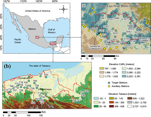
Fig. 1 Considered climatic gauge stations in the analysis of the missing value estimation. (a) Semi-arid region: Upper Laja River Basin (CARL) in the northern part of Guanajuato. (b) Humid region: Tabasco. Cyan circles indicate the target stations within the study regions, and yellow circles mark auxiliary stations adjacent to the study regions. Each station is labeled with the initial S in CARL or T in Tabasco.
Tabasco locates in the southern region of Mexico (Fig. 1b), in the wettest part of the country, and extends from the coastal plain of the Gulf of Mexico to the mountain ranges of northern Chiapas. It is bounded by the states of Campeche, Chiapas, and Veracruz and by the Republic of Guatemala to the east. Tabasco has an area of 25,267 km2, representing 1.3% of Mexican territory. A significant part of the state is a plain, with a few relatively low elevations (400-900 m) in the south (5.84% of the state area). Tabasco is in a tropical zone close to the Gulf of Mexico, which derives in a warm climate with few temperature variations throughout the year. The average yearly temperature is 27 ºC, with an average range from 18.5 to 36 ºC. The average annual precipitation in the state is ~2,190 mm/year in the analysis period, making it the state with the highest annual precipitation in Mexico.
Daily precipitation data from 1993 to 2017 for the semi-arid region and from 1980 to 2012 for the humid region were obtained from the repository of the Comisión Nacional del Agua (CONAGUA) and Servicio Meteorológico Nacional (SMN) (SMN, 2020). We excluded meteorological stations with more than 25% missing data, as recommended by several authors (Dong and Peng, 2013; Morales et al., 2019).
Within the semi-arid region (CARL), we considered 23 target meteorological stations within the region, as well as 24 auxiliary stations adjacent to the basin, which were added to improve the performance of the imputation methods (Fig. 1a). Table I presents the geographic locations, elevation, percentage of missing data, and annual mean precipitation of the target and auxiliary meteorological stations in the CARL.
Table I Latitude, longitude, elevation, percentage of missing data, and annual mean precipitation of the meteorological stations in the CARL (semi-arid region).
| Target stations (Data range from 1993 to 2017) | Auxiliary stations (Data range from 1993 to 2017) | ||||||||||
| Station | Long. | Lat. | Elevation [m] | Precipitation [mm/year] | % missing data | Station | Long. | Lat. | Elevation [m] | Precipitation [mm/year] | % missing data |
| S011 | -100.89 | 20.95 | 2062 | 895.94 | 1.68 | S004 | -101.32 | 20.82 | 1800 | 431.84 | 10.05 |
| S015 | -100.33 | 21.13 | 2114 | 432.57 | 12.39 | S007 | -101.23 | 20.99 | 2357 | 776.73 | 0.36 |
| S017 | -100.95 | 21.15 | 1937 | 467.01 | 0.04 | S024 | -101.27 | 21.02 | 1999 | 728.28 | 0.26 |
| S033 | -100.82 | 20.84 | 1850 | 611.40 | 0.21 | S025 | -101.71 | 21.23 | 1920 | 764.59 | 1.01 |
| S042 | -100.64 | 21.04 | 2009 | 504.98 | 13.02 | S040 | -101.67 | 21.20 | 1865 | 698.50 | 0.25 |
| S049 | -101.42 | 21.21 | 2247 | 657.78 | 4.33 | S041 | -101.15 | 20.68 | 1768 | 571.70 | 7.24 |
| S051 | -100.87 | 21.10 | 1906 | 506.09 | 0.73 | S045 | -101.64 | 21.23 | 2221 | 736.51 | 1.69 |
| S053 | -100.49 | 21.22 | 2206 | 472.91 | 13.03 | S048 | -100.84 | 20.71 | 1933 | 583.55 | 5.67 |
| S061 | -101.21 | 21.46 | 2090 | 459.39 | 17.98 | S050 | -101.48 | 21.65 | 2253 | 466.60 | 0.83 |
| S065 | -100.91 | 21.47 | 2100 | 512.59 | 19.63 | S063 | -101.54 | 21.51 | 2123 | 515.78 | 21.03 |
| S066 | -100.51 | 21.29 | 2041 | 536.48 | 6.84 | S071 | -101.43 | 20.94 | 1768 | 634.28 | 0.01 |
| S070 | -101.19 | 21.07 | 2552 | 669.37 | 3.70 | S082 | -100.22 | 21.21 | 1759 | 438.05 | 14.97 |
| S085 | -101.06 | 20.83 | 2241 | 673.82 | 4.34 | S083 | -100.09 | 21.30 | 1318 | 573.69 | 0.00 |
| S107 | -101.10 | 21.32 | 2003 | 538.81 | 19.03 | S103 | -101.26 | 21.03 | 2147 | 708.74 | 7.71 |
| S121 | -101.06 | 20.92 | 1935 | 607.76 | 8.66 | S122 | -100.62 | 20.76 | 1992 | 629.63 | 2.03 |
| S140 | -101.13 | 21.26 | 2115 | 507.31 | 5.48 | S124 | -101.24 | 20.87 | 1853 | 665.89 | 0.00 |
| S141 | -101.24 | 21.17 | 2475 | 895.94 | 3.22 | S131 | -101.41 | 21.56 | 2198 | 374.73 | 14.0 |
| S144 | -100.43 | 20.91 | 2201 | 362.34 | 11.39 | S135 | -101.40 | 21.10 | 1992 | 661.84 | 19.47 |
| S155 | -100.59 | 20.97 | 2041 | 470.68 | 20.65 | S136 | -101.01 | 20.67 | 1828 | 677.12 | 7.57 |
| S161 | -100.66 | 21.45 | 2192 | 419.78 | 6.69 | S148 | -100.61 | 20.67 | 2019 | 613.05 | 1.98 |
| S167 | -100.38 | 20.99 | 2134 | 450.51 | 6.15 | S153 | -101.55 | 21.11 | 1912 | 625.98 | 18.63 |
| S168 | -100.72 | 20.89 | 1780 | 734.63 | 0.22 | S226 | -100.05 | 20.79 | 1913 | 456.32 | 18.99 |
| S241 | -100.55 | 20.81 | 2375 | 580.69 | 21.27 | S245 | -100.46 | 20.70 | 1885 | 568.03 | 25.0 |
| S493 | -100.57 | 21.67 | 1780 | 375.96 | 9.18 | ||||||
For the humid region (in Tabasco), we analyzed 29 meteorological stations within the region (Fig. 1b). There were 13 auxiliary stations in the area surrounding the region, and only 8 had sufficient records during the period of analysis, which is only ~30% of the target stations. Furthermore, the average distance between auxiliary and target stations was ~70 km. Therefore, we decided not to include the auxiliary stations in this region. Table II presents the geographic locations, elevation, percentage of missing data, and annual mean precipitation of the target meteorological stations in Tabasco.
Table II Latitude, longitude, elevation, percentage of missing data, and annual mean precipitation of the target meteorological stations in Tabasco (humid region).
| Target stations (Data range from 1980 to 2012) | |||||||||||
| Station | Long. | Lat. | Elevation [m] | Precipitation [mm/year] | % missing data | Station | Long. | Lat. | Elevation [m] | Precipitation [mm/year] | % missing data |
| T02 | -92.80 | 18.42 | 3 | 1343.7 | 12.71 | T39 | -93.28 | 18.00 | 23 | 1943.7 | 5.22 |
| T04 | -91.49 | 17.45 | 14 | 2289.4 | 2.22 | T40 | -91.16 | 17.79 | 44 | 1595.7 | 3.28 |
| T06 | -91.28 | 17.64 | 50 | 1689.8 | 2.81 | T42 | -92.78 | 17.46 | 44 | 3418.2 | 4.85 |
| T07 | -93.62 | 18.00 | 12 | 2001.2 | 15.23 | T44 | -92.95 | 17.55 | 51 | 3241.3 | 1.24 |
| T08 | -93.38 | 18.00 | 25 | 2059.4 | 12.24 | T47 | -91.43 | 17.47 | 22 | 2130.1 | 24.00 |
| T09 | -93.22 | 18.25 | 15 | 1733.5 | 19.51 | T50 | -92.60 | 18.38 | 2 | 1518.0 | 5.40 |
| T11 | -92.80 | 17.61 | 20 | 2855.5 | 10.21 | T54 | -92.93 | 18.00 | 24 | 1946.3 | 5.86 |
| T15 | -93.94 | 17.84 | 7 | 2280.7 | 24.9 | T60 | -93.77 | 17.97 | 11 | 1973.9 | 12.64 |
| T19 | -92.81 | 17.72 | 14 | 2562.1 | 1.41 | T61 | -92.92 | 17.51 | 86 | 3639.5 | 16.41 |
| T21 | -91.29 | 17.76 | 29 | 1964.5 | 20.04 | T70 | -92.75 | 17.38 | 63 | 3176.3 | 1.64 |
| T30 | -92.61 | 17.76 | 11 | 2322.8 | 0.68 | T75 | -93.57 | 18.11 | 10 | 2303.4 | 10.23 |
| T34 | -93.21 | 18.40 | 6 | 1622.9 | 8.84 | T76 | -93.50 | 18.11 | 13 | 2271.9 | 24.02 |
| T36 | -93.18 | 18.07 | 15 | 1920.5 | 3.14 | T77 | -93.63 | 18.07 | 12 | 2104.2 | 13.46 |
| T37 | -93.88 | 17.85 | 21 | 2069.1 | 2.14 | T78 | -93.50 | 18.02 | 19 | 1769.7 | 6.16 |
| T84 | -93.02 | 18.17 | 10 | 1735.7 | 6.84 | ||||||
2.2 Missing values interpolation methods
2.2.1 NR and NRWC Methods
A common method for the imputation of missing data is the Normal Ratio Method (NR), modified by Young (1992) to the Normal Ratio with Correlation (NRWC). The estimated value V 0 for the missing data is considered to be a combination of observations with different weights, i.e., V 0 = (∑n i=1 W i V i ) / (∑n i=1 W i ), where W i is the weight of the th nearest meteorological gauge station, W i is the number of nearby meteorological gauge stations, and V i is the corresponding observation. Weights for the surrounding stations used in the estimation algorithm were calculated according to Eq. (1):
Where r i represents the correlation coefficient between the target station and the ith neighboring station, and n i is the number of points used to calculate the correlation coefficient (Xia et al., 1999; Sattari et al., 2017; Kanda et al., 2018).
2.2.2 IDW Method
Another method widely used for estimating missing values in hydrology and climatology is the Inverse Distance Weighting Method (IDW) (Radi et al., 2015; Kamaruzaman et al., 2017; Sattari et al., 2017; Kanda et al., 2018; Morales et al., 2019). IDW estimation of values, based on an observation, is given by Eq. (2):
where θ t is the target station estimation, n the number of neighboring stations used in the interpolation, θ t is the observation at station i, d it is the distance from the neighboring station i to the target station t, and k is the power parameter, most commonly set to 2, 3 or 4 (Teegavarapu and Chandramouli, 2005; Ford and Quiring, 2014). IDW has been further modified by several authors, mainly by adjusting the calculation of distance and weighting factors to enhance the outcomes.
2.2.3 CCW Method
Teegavarapu and Chandramouli (2005) proposed improvements to the IDW method by replacing the weighting factor with the correlation coefficient, as follows in Eq. (3):
where r it is the coefficient of correlation (i.e., the ratio of covariance of two data sets to the product of standard deviations of each data set), derived from all available historical time series data between the data at target station t and their corresponding values recorded at any other neighboring station . Teegavarapu and Chandramouli (2005) named this new method the Correlation Coefficient Weighting Method (CCW) and showed that it was superior to the traditional IDW method for interpolating missing rainfall values.
2.2.4 MCCW Method
Suhaila et al. (2008) presented several modifications to estimate missing precipitation data from the weighting factors of the NR, IDW, and CCW methods. One of them was the Modification of the Correlation Coefficients Weighting Method (MCCW), in which they changed the weighting function of the CCW method proposed by Teegavarapu and Chandramouli (2005), as shown in Eq. (4):
where r it represents the correlation coefficient of the daily precipitation data between the target station t and the th neighboring station; N is the length of the precipitation time series, and p is a parameter between 2 and 6. Larger values of p assign a greater influence to the values closer to the target station. The most commonly used value for p is 2, according to Suhaila et al. (2008).
2.2.5 CIDW Method
Another modification was the Modified Correlation Coefficient with Inverse Distance Weighting Method (CIDW), which is the consequence of combining the IDW and MCCW methods to estimate the missing rain values, as expressed in Eq. (5):
where r p it is the correlation coefficient between the target station t and the ith neighboring station with p between 2 and 6; d it is the distance between target station t and the ith neighboring station. The minimum distances between the target station and neighboring stations strongly influence the IDW method. Still, the correlation factor could also impact the estimation results, so the proposed CIDW method should improve their imputation (Suhaila et al., 2008).
2.2.6 NRIDW Method
The last of the modifications was the Modified Normal Ratio Method with Inverse Distance Method (NRIDW), which was the consequence of combining the IDW with the NRWC proposed by Young (1992). The NRWC method is strongly influenced by positive spatial correlation. At the same time, IDW is affected by the minimum distance between the target station and neighboring stations. Thus, the combination of these weighting factors could improve the outcomes of the estimation of missing values through the weighting factor given by Eq. (6):
The modified methods performed better than the previous versions, according to Suhaila et al. (2008).
2.2.7 NRIDC Method
Azman et al. (2015) presented a combination between NR, IDW, and the correlation value, which they called the Inverse Distance Weighting Method of Normal Ratio with Correlation (NRIDC). This method modified the NRIDW proposed by Suhaila et al. (2008) by including the correlation value. This method keeps the original proposal of combining the normal ratio, the correlation, and the inverse distance in a weighting method, to give more weight to the best estimation to impute missing precipitation data. The weighting of NRIDC is given by Eq. (7):
where r p it is the correlation coefficient between the target station t and the th neighboring station with the best exponent value of p ≥ 4 (Azman et al., 2015); μ t is the sample mean of the data available at the target station t, μ i is the sample mean of the data available at the ith neighboring station, and d it is the distance between the target station t and the ith neighboring station.
2.2.8 HIDW Method
The Altitude Relationship with the Inverse Distance Weighting Method (HIDW) was the consequence of the modification proposed by Golkhatmi et al. (2012). They also modified the IDW by inserting elevation parameters into the weighting function, which was optimized using the genetic algorithm. Its weighting function is:
where h it represents the altitude difference between the target station t and the ith neighboring station, and q and s represent parameters corresponding to distance and elevation, respectively.
2.2.8 GNRIDW and GCIDW Methods
Recently, Morales et al. (2019) proposed two new generalized weighting methods: Generalization of the Modified Normal Ratio Method with the Inverse Distance Method (GNRIDW) and Generalization of the Modified Correlation Coefficient with the Inverse Distance Weighting Method (GCIDW). GNRIDW constitutes a generalization of the NRWC and IDW methods, in which the weighting factors are as follows:
where, in Eq. (9) and Eq. (10), r it , d it and h it represent the correlation coefficient, distance and altitude difference between the target station t and the ith neighboring station, respectively; n i is the length of data, q and s represent parameters corresponding to distance and elevation, respectively. GCIDW constitutes a generalization of the CIDW, IDW, and HIDW. It is also distinguished by the inclusion of free parameters and an altitude factor, as in Eq. (10):
Morales et al. (2019) computed the optimal parameters of Eq. (9) and Eq. (10), employing the adaptation strategy of the covariance matrix.
2.2.9 MICE Method
The Multivariate Imputation by Chained Equations (MICE) package for R software (R Core Team, 2019) implements a procedure that allows the imputation of missing records in a given database. It creates multiple imputations (replacement values) for multivariate missing data based on the Fully Conditional Specification (FCS) method, where each incomplete variable is imputed by a separate model. MICE specifies the multiple imputation model based on each variable for a set of conditional densities P (Y j │X, Y -j ,R, ϕ j ), where Y j is the th column in the data matrix Y, X is a completely observed covariate in the population; Y -j indicates the complement of Y j , that is, all columns in Y except Y j , R is a response indicator of Y, and ϕ j is a parameter. Starting from an initial imputation, it generates imputations by iterating over the conditional densities (van Buuren, 2012). This algorithm can impute blends of continuous, binary, disordered, categorical, and ordered categorical data. To verify the quality of the imputations, the algorithm generates several diagnostic graphs (van Buuren and Groothuis-Oudshoorn, 2011).
The Predictive Mean Matching (PMM) method is built into the MICE package. This is an attractive way to impute multiple missing data of virtually any pattern, especially non-normally distributed quantitative variables (Allison, 2015).
2.2.10 ReddPrec Method
Serrano-Notivoli et al. (2017) presented the ReddPrec package, developed in R software (R Core Team, 2019), and focused on reconstructing daily precipitation. The methodology incorporated in this package creates daily reference values using all data recorded at the closest stations for each targeted day. To do this, multivariate logistic regression is applied based on the data of the ten nearest neighbors, considering the geographic and topographic variables as covariates. This method optimizes all available information; it does not depend on the length of the precipitation series and preserves the local variability of precipitation distribution.
2.2.11 EM Method
Available in SPSS software (IBM Corp, 2017), the Expectation Maximization (EM) algorithm to fill missing data is an interactive method that estimates unknown parameters of a data model. In applying this method, the missing values are initially calculated using the estimated parameters of the model. The method is based on the reciprocal dependency between the model parameters and the missing values. It consists of two steps: the conditional expectation step and the maximization step. In the first step, the conditional expectations of the missing data are calculated given the observed data and the estimates of the model parameters. In the second step, maximum likelihood estimators of the parameters are found by maximizing the expected likelihood of the first step. These steps are repeated until the iterations converge (Schneider, 2001; Firat et al., 2012).
2.2.12 RG Method
Available in SPSS software (IBM Corp, 2017), Linear Regression (RG) is a statistical technique that models the relationship between a response variable and one or more input or predictor variables. The result of regression analysis is often the generation of a model that can be used to estimate or predict future values of the response variable. This technique is widely used partly due to the straightforward interpretation of the desired model, and it is commonly used to impute time series of climatological variables (Jimenez et al., 2014). This method requires two steps: one to estimate the relationship between predictors and missing values and another to use a trend equation to fill in the empty data (Aieb et al., 2019).
2.3 Performance and homogeneity evaluation
2.3.1 Performance indicators
Several indicators have been used in the literature to evaluate the performance of missing data imputation methods. These are the Similarity Index (Suhaila et al., 2008), the Variance Ratio (Ford and Quiring, 2014), the Coefficient of Correlation (Azman et al., 2015), the Coefficient of Determination (Norazizi and Deni, 2019), the Mean Absolute Error (MAE) and the Root Mean Square Error (RMSE). The MAE and RMSE have been the most frequently used indicators (Ford and Quiring, 2014). Although both have been used to evaluate method performance for many years, there has yet to be a consensus on the most appropriate metric for evaluating model errors (Chai and Draxler, 2014). RMSE provides a measure of the mean value of the errors of the estimates. Its outcome is in the units as the original observations. However, this indicator should be avoided when there are large measurement errors since these values significantly affect the result when squared. Therefore, RMSE is considered sensitive to outliers, which is why several authors have rejected it (Willmott and Matsuura, 2005; Willmott et al., 2009). MAE provides an outcome that can be interpreted directly since, like the output of the previous indicator, it has the same units as the original variable (precipitation). Therefore, in this research, we used MAE to compare the performance between different missing data imputation methods since we are using precipitation records without first excluding possible outliers.
The value of the MAE is given by Eq. (11):
where n is the total number of observations, x̑ i is the estimated value, and x i is the observed value related to the corresponding meteorological variable in the target station i.
2.3.2 Homogeneity test of data
Homogeneous climatic series can be defined as those influenced only by climate variations (Firat et al., 2012). Several methods have been proposed to analyze the homogeneity of climatological variables.
The Standard Normal Homogeneity Test (SNHT), the Buishand test, and the Pettitt test assume the null hypothesis that annual values Y i of the test variable Y are independent and identically distributed, as opposed to the alternative hypothesis that a stepwise shift in the mean is present. These tests are able to locate the year where a break is most likely (Wijngaard et al., 2003) to appear. SNHT allows the determination of the inhomogeneous structure at the beginning and/or at the end of the time series (Firat et al., 2012). In contrast, the Buishand range test and the Pettitt test detect a point of change in the observed time series and detect inhomogeneous structures with more sensitivity in the middle of a time series (Firat et al., 2012; Guajardo Panes et al., 2017). The SNHT and the Buishand range tests assume that the Y i values are normally distributed, where Y i (i is the year from 1 to n) is the annual series to be tested, but the Pettitt test does not take into account this consideration (Wijngaard et al., 2003).
SNHT is a likelihood ratio test, and it is performed on a ratio or difference between the candidate station and reference series (Peterson et al., 1998). The comparison of the mean of the first k years of the record with that of the last n - k years is obtained by using the statistic T(k), given by Eq. (12):
where
The Buishand range test can be used with variables having any type of distribution (Guajardo Panes et al., 2017). In Eq. (13), the statistic S * k represents the Buishand test, where Y i (i is the year from 1 to n) is the annual series to be tested, and Y̅ is the mean.
with k = 1,…, n; S * 0 = 0. When the series is homogeneous, the values of S * k will fluctuate around zero, as there are no systematic deviations of the values of Y i with respect to the mean. If a break is present in the year k = K, then, S * k reaches a maximum (negative shift) or minimum (positive shift) near that year. The significance of the shift can be tested through the adjusted range R of Eq. (14):
where s represents the standard deviation (Wijngaard et al., 2003).
The Pettitt test is a non-parametric rank test (Guajardo Panes et al., 2017) that detects a point of change in the observed time series and is more sensitive for detecting inhomogeneous structures in the middle of a time series (Firat et al., 2012). In Eq. 15, the ranges r 1 ,…,r n of each year are used to calculate the statistic X k of the Pettitt test:
with k = 1,…, n. If a break occurs in the year k = E, then the statistic is maximal or minimal near the year k = E:
Wijngaard et al. (2003) and Guajardo Panes et al. (2017) classified stations as reliable or useful, moderately reliable or doubtful, and unreliable or suspect according to the number of tests that rejected the null hypothesis. The reliable class includes the stations for which none or, at most, one of the tests rejected the null hypothesis. The moderately reliable class had the stations for which two tests rejected the null hypothesis, and the unreliable class included those for which the three tests rejected the null hypothesis. The results of each test were evaluated for a significance level of 5%.
2.4 Comparison strategy
To evaluate MAE values in each case, we compared the performance of data imputation methods by first creating a subset of the test data. This subset is selected from all periods in which there are no missing data at the target and auxiliary stations. We used each of the two study regions as a test case to evaluate the imputation methods.
The first case used the target stations (within the region) and auxiliary stations (within 30 km of the region’s border) associated with the semi-arid region (CARL). The period with the fewest missing records was from January 1993 to December 2017. All methods proposed in this study were evaluated to compare their performance in predicting missing values.
The second case used only the target stations within the humid region (Tabasco) (see 2.1 Study area and database for the explanation of stations’ exclusion). The weighting methods were previously compared in the state of Tabasco by Morales et al. (2019), who found that the GCIDW method had the lowest MAE value. Therefore, only the methods EM, GCIDW, MICE, ReddPrec, and RG were evaluated, and their performance was compared. The analysis period from January 1980 to December 2012 was selected to reduce the percentage of missing records.
3. Results and discussion
3.1 Prediction of missing precipitation data
3.1.1 Semi-arid region: Upper Laja River Basin (CARL)
The MAE values of the 23 stations are in Table III, where the lowest MAE values are identified in bold for each imputation method. The ReddPrec method was optimal at nine stations (~39%); GCIDW was optimal at eight stations (~35%); NR was optimal at three stations (~13%), and NRIDC, HIDW, and EM were optimal at 1 station each (~4%). Overall, the weighting methods (led by the GCIDW method) performed best, with average MAE values ≤ 1.60 mm/day. This was followed closely by the ReddPrec method, with an average MAE of 1.63 mm/day. The rest of the methods had MAE values ≥ 2.28 mm/day. It is worth mentioning that the EM and RG methods imputed negative values, and attempting to force these values to zero should be done with caution, as this can modify the mean and shape of the imputed precipitation distribution. In addition, the MAE values of both methods decreased after forcing negative values to zero, but not enough to change the optimal values presented in Table III.
Table III Mean Absolute Error (MAE) values of the imputation methods for precipitation in the CARL (semi-arid region), where the optimal method is highlighted in bold (minimum value of MAE). The units of MAE values are mm/day.
| Station | EM | RG | ReddPrec | MICE | NR | NRWC | CCW | NRIDW | IDW | MCCW | CIDW | NRIDC | HIDW | GNRIDW | GCIDW |
| S011 | 3.40 | 3.90 | 1.68 | 2.71 | 1.91 | 1.54 | 1.67 | 1.55 | 1.77 | 1.50 | 1.48 | 1.49 | 1.77 | 1.51 | 1.46 |
| S015 | 0.13 | 2.35 | 1.51 | 1.73 | 0.91 | 0.87 | 0.86 | 0.90 | 0.86 | 0.86 | 0.90 | 0.91 | 0.86 | 0.86 | 0.83 |
| S017 | 3.31 | 2.48 | 1.87 | 3.02 | 2.19 | 2.23 | 2.21 | 2.19 | 2.17 | 2.19 | 2.17 | 2.16 | 2.17 | 2.17 | 2.17 |
| S033 | 2.62 | 3.54 | 1.89 | 3.01 | 1.77 | 1.61 | 1.63 | 1.60 | 1.62 | 1.60 | 1.59 | 1.59 | 1.58 | 1.58 | 1.58 |
| S042 | 1.95 | 2.35 | 1.26 | 2.25 | 1.31 | 1.23 | 1.23 | 1.24 | 1.24 | 1.22 | 1.24 | 1.23 | 1.24 | 1.23 | 1.22 |
| S049 | 2.26 | 3.16 | 1.30 | 2.37 | 1.63 | 1.39 | 1.66 | 1.33 | 1.31 | 1.31 | 1.31 | 1.29 | 1.31 | 1.31 | 1.31 |
| S051 | 2.39 | 3.29 | 1.21 | 1.60 | 1.46 | 1.41 | 1.45 | 1.42 | 1.53 | 1.40 | 1.40 | 1.40 | 1.53 | 1.39 | 1.39 |
| S053 | 2.12 | 2.81 | 1.03 | 1.85 | 1.23 | 1.18 | 1.18 | 1.27 | 1.20 | 1.17 | 1.25 | 1.22 | 1.18 | 1.15 | 1.11 |
| S061 | 1.84 | 1.81 | 1.06 | 1.55 | 1.09 | 1.32 | 1.33 | 1.35 | 1.35 | 1.25 | 1.27 | 1.26 | 1.22 | 1.22 | 1.22 |
| S065 | 1.94 | 2.22 | 1.04 | 1.78 | 1.24 | 1.24 | 1.26 | 1.26 | 1.30 | 1.24 | 1.26 | 1.23 | 1.15 | 1.14 | 1.14 |
| S066 | 2.56 | 2.59 | 1.29 | 1.81 | 1.39 | 1.30 | 1.37 | 1.50 | 1.42 | 1.21 | 1.21 | 1.21 | 1.42 | 1.30 | 1.21 |
| S070 | 2.65 | 3.70 | 4.12 | 3.56 | 2.26 | 2.26 | 2.33 | 2.23 | 2.46 | 2.21 | 2.21 | 2.21 | 2.46 | 2.22 | 2.18 |
| S085 | 2.18 | 2.29 | 2.07 | 2.35 | 1.69 | 1.86 | 1.83 | 1.87 | 1.86 | 1.82 | 1.87 | 1.87 | 1.86 | 1.85 | 1.82 |
| S107 | 1.97 | 2.44 | 1.34 | 1.81 | 1.47 | 1.31 | 1.50 | 1.26 | 1.26 | 1.26 | 1.26 | 1.22 | 1.23 | 1.19 | 1.16 |
| S121 | 2.12 | 2.94 | 1.47 | 2.36 | 1.84 | 1.87 | 1.89 | 1.84 | 1.89 | 1.85 | 1.84 | 1.82 | 1.76 | 1.76 | 1.76 |
| S140 | 2.23 | 2.21 | 1.25 | 1.98 | 1.48 | 1.41 | 1.61 | 1.29 | 1.28 | 1.27 | 1.27 | 1.27 | 1.27 | 1.28 | 1.27 |
| S141 | 5.48 | 6.06 | 3.70 | 6.37 | 4.02 | 3.32 | 3.32 | 3.30 | 3.29 | 3.32 | 3.29 | 3.29 | 3.29 | 3.29 | 3.29 |
| S144 | 1.98 | 1.60 | 1.26 | 1.90 | 1.40 | 1.53 | 1.59 | 1.45 | 1.40 | 1.38 | 1.38 | 1.38 | 1.40 | 1.34 | 1.33 |
| S155 | 2.31 | 2.35 | 1.09 | 1.97 | 1.46 | 1.39 | 1.40 | 1.43 | 1.43 | 1.36 | 1.41 | 1.36 | 1.29 | 1.29 | 1.29 |
| S161 | 2.07 | 2.25 | 1.55 | 1.52 | 1.37 | 1.29 | 1.32 | 1.28 | 1.37 | 1.27 | 1.27 | 1.27 | 1.37 | 1.28 | 1.27 |
| S167 | 1.44 | 1.50 | 1.07 | 1.07 | 1.06 | 1.17 | 1.19 | 1.17 | 1.26 | 1.17 | 1.17 | 1.17 | 1.25 | 1.17 | 1.17 |
| S168 | 1.87 | 2.19 | 1.81 | 1.88 | 1.48 | 1.52 | 1.51 | 1.53 | 1.49 | 1.51 | 1.50 | 1.50 | 1.49 | 1.51 | 1.49 |
| S241 | 1.85 | 1.98 | 1.72 | 2.08 | 1.25 | 1.43 | 1.42 | 1.45 | 1.42 | 1.42 | 1.44 | 1.41 | 1.26 | 1.24 | 1.22 |
| Average | 2.29 | 2.7 | 1.63 | 2.28 | 1.60 | 1.55 | 1.60 | 1.55 | 1.57 | 1.51 | 1.52 | 1.51 | 1.54 | 1.49 | 1.47 |
Figure 2A1 shows the minimum imputed values of selected methods, in which only RG and EM methods imputed negative values. Negative values do not correspond to the physics of precipitation phenomena, resulting in the suggestion by Teegavarapu (2012) that these methods are not suitable for precipitation.
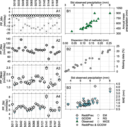
Fig. 2 LEFT (A1 to A4): Comparison of the model-interpolated values and the observed daily precipitation in the CARL (semi-arid region). The comparison is divided into descriptive values as (A1) minimum (PP_Min), (A2) maximum (PP_Max), (A3) mean (PP_Mean), and (A4) standard deviation (PP_Std) of precipitation. RIGHT (B1 to B3): Comparison of key variables with significant Spearman’s rank correlation in Table IV: (B1) annual mean precipitation and dispersion (Std), (B2) missing data and standard deviation of methods (Std of methods), and (B3) Mean Absolute Error and standard observed precipitation of ReddPrec and GCIDW methods, that were selected as representative methods to simplify the analysis.
Table IV Spearman’s rank correlation (rs) applied to annual mean precipitation (Precipitation), percentage of station missing data (% of missing data), meteorological station elevation (Elevation), the standard deviation of observed data (Std [observed data]), dispersion of standard deviation of methods (Dispersion [std of methods]), mean absolute error of methods (MAE method) in the CARL (semi-arid region), where significant correlations have a p-value less than 0.05. NOTE: ReddPrec and GCIDW methods were selected as representative methods to simplify the analysis.
| Key Variables | Test variables | % of missing data | Elevation | Std (observed data) | Dispersion (std of methods) | MAE GCIDW | MAE ReddPrec |
| Precipitation | rs | -0.403 | 0.041 | 0.930 | -0.287 | 0.528 | 0.572 |
| p-value | 0.057 | 0.854 | 0.000 | 0.184 | 0.010 | 0.004 | |
| % missing data | rs | 0.204 | -0.421 | 0.930 | -0.715 | -0.559 | |
| p-value | 0.350 | 0.047 | 0.000 | 0.000 | 0.006 | ||
| Elevation | rs | -0.034 | 0.258 | -0.034 | 0.122 | ||
| p-value | 0.879 | 0.235 | 0.879 | 0.579 | |||
| Std (observed data) | rs | -0.294 | 0.574 | 0.532 | |||
| p-value | 0.172 | 0.005 | 0.010 |
As shown in figure 2A2, there were no relevant differences between maximum imputed and observed values except for station S065, where ReddPrec overpredicted the observed value by 7.9 mm (~10%).
Figure 2A3 shows that the mean precipitation of imputed and observed values had no relevant differences except for the RG method. It is important to note that the mean values of RG and EM methods were evaluated after forcing negative values to zero. Doing so changed the mean annual precipitation from 555 mm/year to 599 mm/year for the RG method and from 553 mm/year to 554 mm/year for the EM method. The RG method generally tended to overpredict the mean observed precipitation in all meteorological stations, with an average difference of ~6.2%.
In addition, in figure 2A4, the standard deviation of the observed and imputed values (negative values of EM and RG methods were forced to zero) among different methods showed appreciable differences at some stations: e.g., S241, S155, S141, S107, S065, S061, S053, S042, and S015. These stations had in common a percentage of missing data greater than 12% (see Table I), except for station S141, which had less than 4% missing data.
Up to this point, it is unclear why certain methods performed better at some climatological stations than others or why the standard deviation of imputed values had larger dispersion between different methods at different stations. We further explored these questions using the GCIDW and ReddPrec methods as representative optimal methods to simplify the analysis.
Spearman’s rank correlation test is a nonparametric approach used to describe the strength and direction of the relationship between two random variables (Lyerly, 1952). In this study, it was applied with key variables and MAE values to identify which variables significantly affected (p<0.05) the performance of GCIDW and ReddPrec methods. Results are provided in Table IV. From this analysis, it is possible to suggest a decrease in methods performance, represented by MAE values, when the dispersion of precipitation data increases (see Fig. 2B3). In addition, the higher the percentage of missing data at the meteorological stations, the greater the dispersion of the standard deviation in the imputed values among different methods (see Fig. 2B2).
Figure 2B1 shows that the increase in mean annual precipitation volume is related to a greater standard deviation of daily precipitation. However, the increase in annual precipitation does not correlate with the rise in elevation.
3.1.2 Humid region: state of Tabasco
The methods EM, GCIDW, MICE, ReddPrec, and RG, were selected to evaluate and compare their performance in a humid region (Tabasco). In this section, auxiliary stations were not considered due to limited availability (see section 2.1).
The MAE values from Table V show that the GCIDW method was optimal in ~59% of the stations (average MAE 6.0 mm/day), EM was optimal in ~24%, and ReddPrec was optimal in ~17%. The RG and MICE methods were not analyzed further because they were not optimal for any station. These numbers confirm a performance reduction of ReddPrec when there are insufficient target stations or auxiliary stations are not considered. However, the EM method (average MAE of 6.5 mm/day) performed better than the ReddPrec method (average MAE of 9.8 mm/day), suggesting that it was not only the inclusion of auxiliary stations that influenced the performance of these methods, but also the precipitation regime.
Table V Mean Absolute Error (MAE) values of the imputation methods for precipitation in Tabasco (humid region), where the optimal method is highlighted in bold (minimum value of MAE). The units of MAE values are mm/day.
| Station | EM | RG | ReddPrec | MICE | GCIDW | Station | EM | RG | ReddPrec | MICE | GCIDW |
| T02 | 5.01 | 6.50 | 6.63 | 5.99 | 4.71 | T40 | 5.22 | 7.98 | 5.98 | 8.20 | 5.22 |
| T04 | 6.92 | 11.93 | 13.74 | 11.74 | 6.07 | T42 | 8.13 | 16.22 | 11.76 | 15.71 | 6.25 |
| T06 | 5.33 | 7.50 | 6.65 | 7.40 | 5.51 | T44 | 5.27 | 16.23 | 9.31 | 15.76 | 4.04 |
| T07 | 6.19 | 11.22 | 5.09 | 10.51 | 6.04 | T47 | 9.43 | 12.42 | 13.29 | 13.00 | 7.52 |
| T08 | 6.80 | 11.46 | 11.28 | 11.28 | 7.97 | T50 | 5.18 | 8.72 | 8.79 | 8.08 | 4.25 |
| T09 | 6.20 | 8.99 | 20.47 | 9.13 | 6.16 | T54 | 5.13 | 10.03 | 6.43 | 9.29 | 5.04 |
| T11 | 9.24 | 14.09 | 9.72 | 14.33 | 7.21 | T60 | 4.91 | 11.01 | 6.18 | 10.42 | 5.03 |
| T15 | 8.29 | 11.81 | 15.44 | 11.59 | 7.45 | T61 | 5.77 | 18.50 | 15.08 | 19.23 | 4.23 |
| T19 | 6.72 | 13.29 | 8.45 | 12.32 | 5.87 | T70 | 7.92 | 15.36 | 12.83 | 14.54 | 6.62 |
| T21 | 7.55 | 10.92 | 6.85 | 10.34 | 6.15 | T75 | 9.04 | 11.90 | 7.06 | 12.37 | 7.61 |
| T30 | 5.74 | 11.87 | 8.33 | 11.47 | 5.77 | T76 | 7.10 | 11.91 | 5.99 | 11.41 | 7.17 |
| T34 | 5.29 | 8.33 | 22.91 | 8.70 | 4.73 | T77 | 9.46 | 10.94 | 8.57 | 12.30 | 8.34 |
| T36 | 7.45 | 10.48 | 6.21 | 10.65 | 5.92 | T78 | 6.59 | 9.70 | 6.07 | 9.10 | 6.85 |
| T37 | 4.88 | 10.16 | 14.91 | 9.09 | 5.25 | T84 | 5.08 | 10.51 | 4.49 | 9.36 | 4.81 |
| T39 | 4.54 | 9.97 | 6.10 | 9.16 | 6.29 | ||||||
| Average | 6.56 | 11.38 | 9.81 | 11.12 | 6.00 |
The EM method predicted negative values (Fig. 3A1) for the semi-arid region. Negative values from the EM and RG methods were forced to zero to evaluate descriptive statistics shown in Figure 3A3 and Figure 3A4. The average MAE value of the EM method decreased to 6.46 mm/day after forcing negative values to zero, but not enough to change the optimal values presented in Table V. Maximum (Fig. 3A2) and mean (Fig. 3A3) precipitation values showed no relevant differences with the observed values, except for standard deviation (Fig. 3A4) at stations T07, T08, T09, T11, T15, T21, T47, T60, T75, T76 and T77, which had a percentage of missing data in the range of 10-24%.
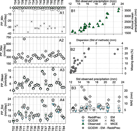
Fig 3 LEFT (A1 to A4): Comparison of the model interpolated values and the observed daily precipitation in Tabasco (humid region). The comparison is divided into descriptive values as (A1) minimum (PP_Min), (A2) maximum (PP_Max), (A3) mean (PP_Mean), and (A4) standard deviation (PP_Std) of precipitation. RIGHT (B1 to B3): Comparison of key variables with significant Spearman’s rank correlation in Table VI: (B1) annual mean precipitation and dispersion (Std), (B2) missing data and standard deviation of methods (Std of methods), and (B3) Mean Absolute Error and standard observed precipitation of ReddPrec and GCIDW methods, which were selected as representative methods to simplify the analysis.
Table VI Spearman’s rank correlation (rs) applied to annual mean precipitation (Precipitation), percentage of station missing data (% of missing data), meteorological station elevation (Elevation), the standard deviation of observed data (Std [observed data]), dispersion of standard deviation of methods (Dispersion [std of methods]), mean absolute error of methods (MAE method) in Tabasco (humid region), where significant correlations have a p-value less than 0.05. NOTE: ReddPrec, GCIDW, and EM methods were selected as representative methods to simplify the analysis.
| Key variable | Test variables | % of missing data | Elevation | Std (observed data) | Dispersion (Std of methods) | MAE GCIDW | MAE ReddPrec | MAE EM |
| Precipitation | rs | -0.126 | 0.341 | 0.930 | 0.013 | 0.291 | 0.373 | 0.506 |
| p-value | 0.515 | 0.070 | 0.000 | 0.948 | 0.125 | 0.047 | 0.006 | |
| % of missing data | rs | -0.250 | -0.005 | 0.793 | 0.345 | 0.038 | 0.312 | |
| p-value | 0.191 | 0.979 | 0.000 | 0.068 | 0.843 | 0.099 | ||
| Elevation | rs | 0.259 | -0.118 | 0.038 | 0.104 | 0.083 | ||
| p-value | 0.176 | 0.543 | 0.846 | 0.591 | 0.668 | |||
| Std (observed data) | rs | 0.043 | 0.343 | 0.283 | 0.526 | |||
| p-value | 0.825 | 0.069 | 0.136 | 0.004 |
The ReddPrec method significantly overpredicted the observed maximum daily precipitation at stations T04, T09, T47, T60, and T76 with a difference of 51-220 mm/day. In addition, the observed mean daily precipitation was overpredicted at stations T09 and T47 with values of 1.15 mm/day and 1.44 mm/day (see Fig. 3A2 and Fig. 3A3), as was the observed standard deviation at stations T09 and T47 with an average difference of ~6 mm/day (see Fig. 3A4).
The GCIDW method predicted the observed maximum and mean daily precipitation with no significant differences (see Fig. 3A2 and Fig. 3A3). Nevertheless, there was a considerable difference with the observed standard deviation of precipitation; the standard deviation of precipitation was underpredicted in 45% of stations, with a difference of 0.5-2.5 mm/day.
The effect of key variables on the performance of the methods is summarized in Table VI, where again, the percentage of missing data has a significant correlation with the dispersion of GCIDW, EM, and ReddPrec standard deviation (Fig. 3B2). Elevation did not have a significant correlation with the MAE values; the explanation is probably due to the low height of the stations, which varies between 2 m and 83 m with an average of 23 m (see Table II).
Annual precipitation volume was significantly positively correlated with the standard deviation of daily precipitation (Fig. 3B1). However, it is impossible to suggest a decrease in performance, represented by MAE values, with increasing precipitation dispersion and missing data percentage (see Fig. 3B3).
3.1.3 Precipitation regime influence over MAE values in the semi-arid and humid regions
Given the results analyzed in the semi-arid and humid regions, where key variables with significant correlation were analyzed separately by climate region, it is also relevant to analyze both climate regions together to show the evolution of MAE values for GCIDW, ReddPrec, EM, MICE, and RG methods in function of the mean annual precipitation of each meteorological station (see Fig. 4).
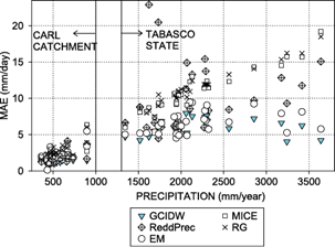
Fig 4 Comparison of the MAE values for selected methods and the annual mean precipitation of meteorological stations in the semi-arid region (CARL) and the humid region (Tabasco).
In Figure 4, it is possible to observe that the performance of the GCIDW and EM methods gradually decreased as the precipitation regime increased, up to a threshold of ~2000 mm/year, at which the performance of these methods stabilizes with a slight tendency to improve. On the other hand, the RG and MICE methods showed a clear tendency to decrease in performance as the annual mean precipitation increases. Finally, there was a significant correlation between the MAE value of the ReddPrec method and the annual mean precipitation (see Table IV and Table VI); however, this linear correlation is less evident in the humid region than in the semi-arid region, especially in the range between 1500-2500 mm/year, where MAE values are higher than 14 mm/day at stations T09, T15, T34 and T37 which visually do not follow a linear correlation (see Fig. 4).
3.2 Homogeneity analysis
In this section, the SNHT, Pettitt, and Buishand range tests were applied to analyze the homogeneity of the precipitation time series, completed with the optimal imputation methods for each analysis region. Each method was evaluated with a confidence level of 95%.
3.2.1 Semi-arid region: Upper Laja River Basin (CARL)
Table VII summarizes the p-values and the years of four stations (17.4%) in which the homogeneity tests detected changes in precipitation, including two stations (S061 and S141) where three homogeneity methods coincided in detecting the year 2001 as the year of change. The year 2001 was also the most frequent in terms of changes in homogeneity. This change in the homogeneity could be related to the modernization of the equipment and instrumentation of the meteorological stations from 2001 to 2006 (CONAGUA, 2012). 78.3% of stations were homogeneous, without changes in precipitation. The homogeneity test was applied individually for 14 imputation methods. The results showed the same number of reliable stations for all 14 but with some differences concerning the year of change in the unreliable or moderately reliable stations.
Table VII Comparison of precipitation homogeneity test results in the CARL (semi-arid region). Only stations where homogeneity tests result in Unreliable or Moderately reliable are shown.
| Station | PETTITT test | SNHT | BUISHAND test | Classification of homogeneity | |||
| p-value | Year of shift | p-value | Year of shift | p-value | Year of shift | ||
| S051 | 0.0270 | 2001 | 0.0193 | 2001 | Moderately reliable | ||
| S061 | 0.0026 | 2001 | 2.2E-16 | 2001 | 0.0003 | 2001 | Unreliable |
| S140 | 0.0336 | 2000 | 0.0199 | 2000 | Moderately reliable | ||
| S141 | 0.0047 | 2001 | 0.0087 | 2001 | 0.0252 | 2001 | Unreliable |
3.2.2 Humid region: state of Tabasco
Table VIII shows p-values and the years of three stations (10.3%) in which the homogeneity tests detected changes in precipitation. Twenty-six stations (89.7%) were classified as reliable, with the precipitation data corresponding to homogeneous conditions.
Table VIII Comparison of precipitation homogeneity test results in Tabasco (humid region). Only stations where homogeneity tests detect a year of change in precipitation are shown.
| Station | PETTITT test | SNHT | BUISHAND test | Classification of homogeneity | |||
| p-value | Year of shift | p-value | Year of shift | p-value | Year of shift | ||
| T75 | 0.0388 | 1995 | 0.0017 | 1995 | Moderately reliable | ||
| T77 | 0.0388 | 2004 | 0.0001 | 2009 | 0.0374 | 2004 | Unreliable |
| T78 | 0.0185 | 1997 | 0.0464 | 1997 | 0.0033 | 1997 | Unreliable |
4. Conclusions
A comparison of 15 missing data imputation methods was presented to analyze their performance in two different climatic and orographic regions. Meteorological stations from a semi-arid region, the Upper Laja River Basin (CARL) in Guanajuato, were used with auxiliary stations outside their limits to improve methods performance. On the other hand, in the humid region, the state of Tabasco, we included only meteorological stations within the region’s limits. Daily preciptation from 1993 to 2017 was used for the semi-arid region and from 1980 to 2012 for the humid region. Stations with more than 25% of missing data were excluded, but possible outliers in the observed data were retained.
In the semi-arid region of the CARL, the methods with the best performance on average were those from the family of weighting imputation methods, which gave the lowest mean MAE values (MAE ≤ 1.6 mm/day), led by the GCIDW method with an average MAE value of 1.46 mm/day. Then the ReddPrec method followed closely with an average MAE value = 1.63 mm/day. The rest of the methods had an average MAE value of ≥ 2.28 mm/day. The RG and EM methods imputed negative values of precipitation. After forcing negative values to zero, the MAE values were reduced (from MAE value ≥ 2.28 mm/day to MAE ≥ 1.9 mm/day). Still, the RG method incremented the average precipitation significantly (from 555 mm/year with negative values to 599 mm/year, forcing negative values to zero). ReddPrec and GCIDW were the optimal methods in nine and eight stations, respectively, out of 23 stations.
The methods EM, GCIDW, MICE, ReddPrec, and RG, were compared in the humid region (Tabasco). In this region, GCIDW was optimal in ~59% of stations, EM in ~24%, and ReddPrec in ~17%, with average MAE values of ~6.0 mm/day, 6.5 mm/day, and ~9.8 mm/day, respectively. ReddPrec performance was significantly lower than GCIDW and EM, where the analysis of results suggested that the performance of the ReddPrecc method decreased considerably with increasing mean annual precipitation, which was exacerbated by the absence of auxiliary stations. In contrast, the EM and GCIDW methods performed better with increasing mean annual precipitation.
From the calculations of both climate regions, a significant correlation was observed between the MAE values and mean annual precipitation in which the methods’ performance was lower in the humid region (Tabasco) compared to the semi-arid region (CARL). The most plausible explanation for this difference is the greater dispersion of mean annual precipitation in Tabasco (1340-3640 mm/year) compared to the CARL (360-900 mm/year). Nevertheless, this analysis did not consider the influence of the sampling error of meteorological stations, which becomes more significant as precipitation increases.
To explore why methods performance increases at some climatological stations and decreases at others, Spearman’s rank correlation was applied between key variables and MAE values of methods. There was a significant negative correlation between the percentage of missing data and MAE values (in the semi-arid region) and a significant positive correlation between precipitation regime and dispersion of predictions between methods (in both climatic regions). Thus, the percentage of missing data and precipitation range have crucial repercussions on the methods’ performance. This suggests that assumptions and methodologies implemented in each imputation method become more relevant when there is more missing data and precipitation dispersion (a higher precipitation regime).
The analysis of homogeneity in different climatic regions confirmed that the optimal missing data imputation methods are adequate to maintain the homogeneity of data, with some differences in the year of the shift in some meteorological stations.

