


 nueva página del texto (beta)
 Inglés (pdf)
 Artículo en XML
 Referencias del artículo
 Enviar artículo por email
 Citado por SciELO
  Similares en
SciELO
Similares en
SciELO 
 Permalink
1. Introduction
As Indonesia is one of the tropical areas with the ability to influence weather conditions globally (Madden and Julian, 1972), many researchers have observed weather dynamics in this region. A previous research by Tsuda et al. (2006) revealed that some atmospheric waves, for instance, the Kelvin wave and other long-period (> 5 days) oscillations, were detected in the middle-level to upper-level troposphere over Indonesia. Furthermore, a predominance of Kelvin waves over Indonesia was also revealed by Kiladis et al. (2009). Another study suggested that the Madden Julian Oscillation (MJO) triggers Indonesian rainfall variability, proven by a strong correlation of rainfall distribution during each MJO phase over the Indonesian region (Hidayat and Kizu, 2010). Sobel and Maloney (2013) considered the MJO as a “moisture mode” rather than a wave, where its formation depends on the prognostic humidity equation, therefore only occurs in a humid atmosphere. Meanwhile, prior studies suggested that MJO occurs in both wet and dry atmosphere, which represent peak and trough phases of the wave characteristic (Wheeler and Kiladis, 1999; Wheeler and Hendon, 2004). Moreover, Wheeler and Kiladis (1999) revealed that MJO is a phenomenon that oscillates at a low frequency and low wavenumber, but not along any theoretical equatorial wave dispersion curves as in convectively coupled equatorial waves (CCEW). It has also been suggested that both MJO and Kelvin waves over Indonesia are strongly correlated with the Australian-Indonesian monsoon (Wheeler and McBride, 2005). It is widely recognized that latent heat released by tropical precipitation can drive a strong interaction up to the level of large-scale atmospheric circulation (Holton, 2004). As large-scale weather phenomena, equatorial waves including MJO play a significant role in the tropics, particularly over Indonesia.
The theories regarding equatorial waves using shallow water equations have rapidly developed since they were first investigated by Matsuno (1966), who defined the equations from motion and mass conservation. A couple of decades later, global monitoring and prediction of MJO and CCEW were introduced by Wheeler and Weickmann (2001) based on the Fourier method to filter various modes of synoptic to intraseasonal variability for each specific characteristic of zonal wavenumbers and frequencies. The study of Maharaj and Wheeler (2005) into predicting MJO used the vector autoregressive (VAR) method, applied to all phases of real-time multivariate MJO series 1 (RMM1) and series 2 (RMM2). Meanwhile, another statistical method for predicting MJO was developed by Jiang et al. (2007) using a multivariate lag-regression model for two lead principal components. In contrast, the numerical weather prediction (NWP) model was not able to prevent large errors in predicting equatorial waves coupled with convection (Zagar et al., 2005). Thus, statistical methods have been relied upon to provide better accuracy than NWP in terms of equatorial-wave prediction models (Wheeler and Weickmann, 2001). Therefore, comparison of the statistical autoregressive (AR) method with equatorial-wave data filtered from the NWP prediction model is necessary to achieve a more accurate MJO and CCEW forecasting method. A localized domain was required to achieve the best results, and so the complexity of the Indonesian archipelago was therefore selected to be the focus area for this study (Ramage, 1971).
The first objective of this study is to seek improved forecasting skills for predicting MJO and CCEW over Indonesia, achieved by comparing statistical AR for rainfall-rate estimation data with the NWP product. AR(1) and AR(2) methods were calculated, but only AR(2) will be described in detail for the reason described in the results section. The NWP product used in this study was the European Centre for Medium-Range Weather Forecasts (ECMWF) Re-Analysis Interim (ERA-Interim) short-range precipitation forecast model, filtered into MJO and CCEW using a space-time spectral analysis method. The second objective of this research is to provide an assessment of the statistical AR method for predicting MJO and CCEW in Indonesia using Tropical Rainfall Measuring Mission (TRMM) data and the NWP model product drawn from the ERA-Interim precipitation forecast data.
2. Data and methods
2.1 Data
A 13-year series of daily TRMM data (3B42 V7 derived) was filtered for MJO and CCEW atmospheric phenomena, divided into two datasets. The first dataset was the 10-year period from January 1, 2006 to December 31, 2015 used for the AR model process, while the second was a 1-year dataset for 2016, used for AR prediction for the same 1-year period. A similar dataset clustering method was used to apply two consecutive years through 2018, i.e., the first dataset was 2007 to 2016 and the second was 2017, as well the first dataset was 2008 to 2017, and the second was 2018. The three latter datasets (2016 to 2018) were then used to verify the final results of statistical AR and the ERA-Interim precipitation forecast in this study. The use of TRMM was considered for several reasons, such as continuous data acquisition, finer resolution (0.25º × 0.25º), comprehensively merged infrared-microwave multi-satellite, and the collection and conversion of all available data into precipitation estimates (see Huffman et al. [2006] for more detailed documentation.)
Meanwhile, a similar long period of total precipitation drawn from ECMWF ERA-Interim precipitation forecasts was used to filter for MJO and CCEW, also divided into two datasets. The first dataset comprises daily total precipitation (summed 12-hourly) from ERA-Interim reanalysis data for the period from January 1, 2006 to December 31, 2016, while the second dataset encompasses daily total precipitation from the ERA-Interim forecast model (ds.627) for the 1-year period from January 1 to December 31, 2016. A clustering dataset similar to the statistical AR method was attempted for two consecutive years (2017-2018) in order to obtain the forecast skill for the same period. Both the ERA-Interim reanalysis and forecast datasets were used to filter for MJO and CCEW phenomena and were then utilized for prediction assessment for the years 2016-2018. A different resolution for the ERA-Interim reanalysis and forecast dataset was encountered, using a 0.75º grid for the reanalysis dataset and a 0.703º × ~0.702º grid for the forecast dataset (see Dee et al. [2011] for the ERA-Interim dataset and the ERA report series for ERA-Interim archive v. 2.0 from the ECMWF documentation [Berrisford et al., 2011]).
2.2 Method
A uniform spatial resolution for all datasets was required to simplify the computational mathematical process using the inverse distance weight method. The 0.5º grid resolution was applied to the daily 3B42 dataset, while the 0.75º grid was applied to the ERA-Interim dataset. The main benefit of this method is the reduction of delays and costs in running the mathematical equations for very large datasets. Meanwhile, to filter all datasets into the MJO and CCEW atmospheric phenomena, the space-time spectral analysis derived from Wheeler and Kiladis (1999) (hereafter known as WK99) was used to obtain information for trapped waves at the equator based on each wave’s characteristic. This method was performed by converting the time-space domain into a frequency-wavenumber domain, in which each wave has a specific frequency-wavenumber domain. The zonal wavenumber (k) applied in this study was between -20 and 20 for the whole equatorial globe with a latitudinal window (ϕ) between 20º N and 20º S; the equivalent depth (ℎe) applied in this study was from 8 to 90 m.
The interannual variability that arises in conjunction with the maturing of El Nino-Southern Oscillation (ENSO) over the dateline/Maritime Continent has proven to be able to mask the real signs of MJO (Wheeler and Hendon, 2004) and so the removal of this factor was necessary. On the other hand, Liu et al. (2017) suggested that the Indian Ocean Dipole (IOD) is strongly correlated rather than ENSO to the MJO forecast skill. Nevertheless, due to the barrier effect constraint of the MJO during the passing of the Indo-Pacific Maritime Continent (Zhang and Ling, 2017; Chen et al., 2020), which has a significant connection with the IOD (Liu et al., 2017), the calculation in this paper accounts only for the ENSO influence. A 13-year weekly Nino3.4 index from the National Oceanic and Atmospheric Administration was used to apply daily regression against daily precipitation of 3B42 and ERA-Interim reanalysis and forecast models. Simple linear interpolation was applied to the weekly Nino3.4 index to obtain a daily Nino3.4 index. The daily regression value for ENSO variability was then removed from all daily data related to MJO. The Nino3.4 index was selected because its locus represents the sea surface temperature anomaly over the dateline, where the mature phase of ENSO occurs.
To perform MJO and CCEW prediction statistically from 3B42 dataset a simple AR method in the form of Eq. (1) (Wilks, 2006) was applied without any modification but selecting only for order values (i.e., the order of 1 and 2):
where X t+1 is the next value in the time series or the next predicted value, X t+1 - μ is the anomaly of the next predicted value, K is an autoregressive order which is also a weighted sum of the previous K anomalies, ε t+1 is a residual or a random component, Øk is the autoregressive coefficient, and μ is the mean of the time series.
Estimated data for daily precipitation from the first (2006-2015), the second (2007-2016) and the last 3B42 10-year datasets (2008-2017) was filtered to capture signals for each wave using the WK99 method. These data was then used as model fitting for each grid. The aim of splitting the process into three 10-year periods was to make a more equal filtering process within the transformation of space-time into the frequency-wavenumber during a filtering process for each period. Another aim was to facilitate each year’s (from 2016 to 2018) evaluation (though not shown and described in this paper). The three 10-year 3B42 datasets were filtered using the same method and were then used as past data for forecasting the future value of each grid. After the AR(1) and AR(2) models had been fitted for each grid of the three 10-year datasets, a forecast process was applied using each model fit and past data for each grid. This process was repeated for each day from January 1 to December 31, 2016 and consecutively for the next two years for forecast leads of 1 to 7 days. The process is marked for each grid as ForecastDAY(model_fit, past_data, forecast_lead) in Figure 1. AR(1) was also tested for the 3B42 dataset in this study, but as it compared poorly with AR(2) in forecast calculations (figures not shown) it will not be described further in detail.

Fig. 1 Schematic representation of the filtered 3B42-AR process to forecast MJO and CCEW at a certain grid and certain day for 1- to 7-day forecast leads (vertical solid gray arrow) using model fitting (solid gray line) and past data (dashed black line). The forecast process covers January 1, 2016 to December 31, 2018.
Meanwhile, to assess daily precipitation forecasts from ERA-Interim data related to MJO and CCEW, the corresponding data period to the daily 3B42 dataset was selected for daily total precipitation from the ERA-Interim data. The data-filtering process using the WK99 method was applied from January 1 to December 31, 2016 for two clustered datasets, as already mentioned. A similar method was also applied for the periods 2007-2017 and 2008-2018. The three 10-year ERA-Interim reanalysis datasets were combined with the 1-year ERA-Interim forecast-model dataset for 2016, 2017 and 2018, consecutively. Daily repetitions of wave filtering were applied to the actual initial forecast times, from January 1 to December 31, 2016 as well for the next two consecutive years, using a combined dataset consisting of the 10-year reanalysis dataset and the 1- to 7-day forecast leads for the same period. The last filtered day for each 1-year iteration, which was a filtered ERA-Interim precipitation forecast dataset, was then collected into the 2016, 2017, and 2018 filtered ERA-Interim precipitation forecast data. Thus, 1096 days (from 2016 to 2018) of iterating filter processes were run to obtain 1- to 7-day forecast leads by employing ERA-Interim total precipitation forecast data (Fig. 2).
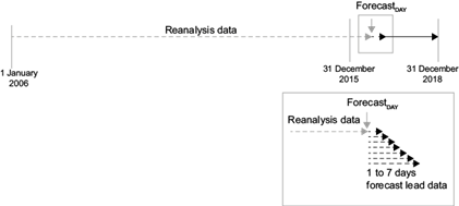
Fig. 2 Schematic representation of the filtered ERA-Interim precipitation forecast process for MJO and CCEW using a precipitation reanalysis dataset (dashed gray line) and precipitation forecast model dataset of 1- to 7-day forecast leads (dashed black line) to forecast at a certain day for 1- to 7-day forecast leads (vertical solid gray arrow) using the WK99 filtering method. The forecast process time period is the same as in Figure 1.
Furthermore, a verification process was performed using a 3-year 3B42 daily precipitation dataset from January 1, 2016 to December 31, 2018. As 3B42-TRMM is a good proxy for real precipitation on the surface, it was therefore employed to evaluate both forecast calculations (Huffman et al., 2006; Irfan et al., 2019). To adjust the initial time of the verification process to the prediction process, a full 2006-2015 dataset combined with the 2016 dataset was run to obtain the last day analysis of MJO and CCEW atmospheric data as if in the real operational mode. The same method was applied to the next two batch periods consecutively. Then, the 1096 days of analyzed data for each filtered wave were compared to 1096 days of forecast data obtained from the previous prediction processes for both the 3B42-TRMM and the ERA-Interim precipitation forecast datasets, in order to identify the accuracy for both processes. Since the calculation (especially for the statistical method) was more independent for one grid based on the previous dataset as historical data in a certain grid point, the verification result between the summer and winter seasons was not distinguished in this paper. Another reason is that this paper aimed to point out the comparison between two methods, thus we ruled out both the phases and the seasons
3. Results
Three years (2016 to 2018) were selected to examine the forecasting accuracy of both processes using the verification calculation equations already described. Figure 3 shows the various sensitivities of the filtered 3B42-AR(2) forecast using a correlation between the filtered 3B42-AR(2) process and the filtered 3B42 data for each wave. Figure 3 shows that the highest forecasting efficiency of the filtered 3B42-AR(2) calculations was for MJO forecast results, in which the maximum correlation reaches 0.99 over East Nusa Tenggara at day +1, and settled at a correlation coefficient of more than 0.9 until day +7, as clearly indicated in Figure 5a. Although the lowest correlation pattern was located over the most equatorial Indonesian region, the correlation coefficient value was still greater than 0.9. The results of Kelvin wave forecast filtered 3B42-AR(2) calculations exhibit the lowest forecast skill, where the correlation coefficient weakens until day +4 and then slightly rises from day +5 through day +7, as shown in figure 5-a. Figure 3-b indicates that most of the Indonesian region, particularly over the southern hemisphere and equator, exhibit the highest correlation pattern during day +1 and then weakens during day +2. Nevertheless, the correlation coefficient indicates below 0.5 and even reaches a negative value over Sumatra and Borneo at day +2 forecast lead.
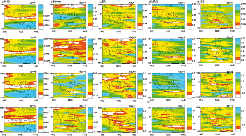
Fig. 3 Geographical correlation between the filtered 3B42-AR(2) process and the filtered 3B42 observations for (a) MJO, (b) Kelvin, (c) ER, (d) MRG, and (e) IG1, at 1- to 7-day forecast leads (top to bottom).
Other satisfactory results of the filtered 3B42-AR(2) process are exhibited by Equatorial Rossby (ER), Mixed Rossby-Gravity (MRG), and inertia-gravity data in zonal wavenumber 1 (IG1), as shown in Figure 5a. However, from the same figure, the ER forecast results indicate a slightly weakening lapse compared with MRG and IG1. The last two waves even reach a negative correlation value during day +5 through day +7, as shown in Figure 3d, e. In spite of this, there is a strong coefficient correlation pattern for ER over southern Papua, with the weak correlation predominantly occuring in the Indonesian region particularly over northern Sumatra and southern Sulawesi during day +5 through day +7 (Fig. 3c). Furthermore, Figure 3d indicates that a weak correlation locus is present in the most southerly part of the Indonesian region, particularly over Bali, West Nusa Tenggara and East Nusa Tenggara during day +1 through day +7 for MRG. Even though a higher correlation was observed over the northern part of Indonesia during day +3 through day +5, the correlation coefficient value is still less than 0.7 at day +3 and less than 0.3 at day +5. Figure 3e shows a strong correlation that appears to be predominant over Indonesia at day +1. However, a lower correlation coefficient is observed over southern Borneo as well as over central and southern Sulawesi at day +3 and continues to weaken until day +7.
Figures 3 and 5a show that the forecasting accuracy results obtained from the correlation coefficients between filtered 3B42-AR(2) calculations indicate a daily weakening trend. The results seem to be different for the forecasts obtained for the filtered ERA-Interim precipitation, where a persistent trend is exhibited from day +1 through day +7 for all waves, as shown in Figures 4 and 5b, both of which show that the correlation coefficient values for each wave, particularly for MJO, ER, MRG, and IG1, are weaker than the correlation coefficient values obtained from the filtered 3B42-AR(2) calculation. However, a consistent correlation without reaching negative values makes this process more reliable in the later forecast lead times than the filtered 3B42-AR(2) process, except for the IG1 result, which will be described later. This persistent trend is presumably due to a consistent distribution pattern of total precipitation for each different lead time from the ERA-Interim precipitation forecast model, even though there is a discrepancy of precipitation-value distribution for each forecast lead. Thus, wavenumber and frequency domain gathered from this consistent oscillation pattern from the ERA-Interim precipitation forecast model were then filtered and classified as MJO and CCEW wave characteristics using the WK99 filter method.
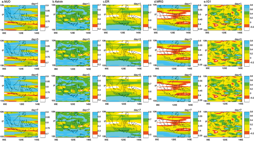
Fig. 4 As in Figure 3 but for the filtered ERA-Interim precipitation forecast process against the filtered 3B42 observation dataset.
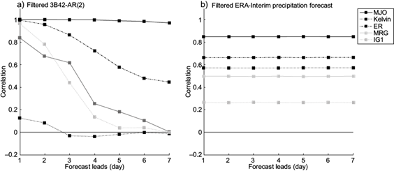
Fig. 5 Temporal correlation between (a) the filtered 3B42-AR(2) process and the filtered 3B42 observation dataset and (b) the filtered ERA-Interim precipitation forecast process against the filtered 3B42 observation datasetfor MJO, Kelvin, ER, MRG, and IG1 (indicated by different line patterns) at 1- to 7-day forecast leads.
Moreover, a moderate correlation (more than 0.5) is observed over most of the Indonesian region, particularly for MJO, Kelvin waves, and ER forecast results. However, a weak correlation is still observed over the western and eastern part of Papua, central Sumatra, and southern Sulawesi for Kelvin waves (Fig. 4b) and over the most equatorial Indonesian region for ER (Fig. 4c). A less significant correlation seems to be predominant over Indonesia for MRG forecast results, which still indicates a positive correlation (Fig. 4d), but seemingly less reliable if compared to the filtered 3B42-AR(2) calculation, where the correlation is higher than 0.6 during day +1 through day +3, as shown in Figure 3d. Meanwhile, a negative correlation is observed over most of the Indonesia area, particularly over southern Sulawesi, Bali, West Nusa Tenggara, and the southern part of Papua (Fig. 4e), making the filtered ERA-Interim precipitation forecast process less reliable as a forecasting calculation for IG1 when compared with the filtered 3B42-AR(2) calculation, particularly at day +1 (Fig. 3e).
The root mean square error (RMSE) was then calculated to obtain an error value for providing another forecasting accuracy assessment in addition to the correlation coefficient method. From Table I, we notice that the RMSE average for all waves continues to increase from day +1 through day +2, with a daily RMSE mean of approximately 0.14 for the filtered 3B42-AR(2) process. Meanwhile, a constant RMSE mean for all waves from day +1 through day +7 is revealed for the filtered ERA-Interim precipitation forecast calculation, which is coherent with Figures 4 and 5 for the reason already mentioned. Nevertheless, there is a greater RMSE for the filtered 3B42-AR(2) calculation as compared to filtered ERA-Interim precipitation forecast calculations for each day, with an RMSE mean difference of approximately 1.21 from both calculations for each day. This means that residuals (prediction errors) for the filtered AR(2) calculation seem to be larger than for the filtered ERA-Interim precipitation forecast calculation; thus, using a filtered ERA-Interim precipitation forecast process is preferable for reducing errors in predicting MJO and CCEW over Indonesia in terms of different forecast leads. Furthermore, Table II shows that a greater residual RMSE is also exhibited for the filtered 3B42-AR(2) calculation compared with the filtered ERA-Interim precipitation forecast calculation, as indicated by the RMSE of each different wave averaged for 1- to 7-day forecast leads. Thus, a filtered ERA-Interim precipitation forecast process is the most reliable calculation process for MJO and CCEW when compared with the filtered 3B42-AR(2) process. RMSE results for both processes indicate that if errors are averaged for all different waves (Table I) or for all different forecast leads (Table II), a better forecast accuracy is achieved for filtered ERA-Interim precipitation forecast calculations. On the other hand, a higher correlation is gained for all wave types (except Kelvin waves) at the beginning of forecast leads, except for MJO, which is consistent at a higher magnitude at all forecast leads with the filtered 3B42-AR(2) calculation (Fig.5-a).
Table I RMSE for the filtered 3B42-AR(2) process as predicted values against the filtered 3B42 observation dataset as observed values, and the filtered ERA-Interim precipitation forecast process as predicted values against the filtered 3B42 observation dataset.
| day +1 | day +2 | day +3 | day +4 | day +5 | day +6 | day +7 | |
| AR(2) | 0.85 | 1.10 | 1.32 | 1.54 | 1.63 | 1.69 | 1.72 |
| ERA | 0.20 | 0.20 | 0.20 | 0.20 | 0.20 | 0.20 | 0.20 |
(AR)2: statistic autoregression method 2; ERA: ERA-Interim reanalysis.
In addition, the Taylor diagram was also examined in this study to evaluate the forecast skill, both for filtered 3B42-AR and for filtered ERA-Interim precipitation forecasts. The Taylor diagram was developed by Taylor (2001) to assess different model skills in terms of their correlation, RMSE and standard deviation. The MJO forecast skill from filtered 3B42-AR(2) calculations in Figure 6 shows the highest correlation (> 0.95) and weakest RMSE (< 1), which also lies close to the reference standard deviation. On the other hand, the Kelvin wave shows the lowest correlation of about less than 0.2, a relatively high RMSE (< 3) and the greatest standard deviation difference compared to other waves. Meanwhile, the ER coefficient correlation and RMSE show a constant degradation and a constant increase, respectively, from day +1 through day +7. However, the ER has a similar standard deviation between the filtered 3B42-AR(2) output and the reference. MRG and IG1 also exhibit a constant decrease of the correlation coefficient and a constant increase of RMSE and the standard deviation difference from the reference. ER and IG1 show a similar pattern except for the beginning forecast time, where IG has a higher coefficient correlation of about 0.95 and standard deviation closer to the reference than MRG.
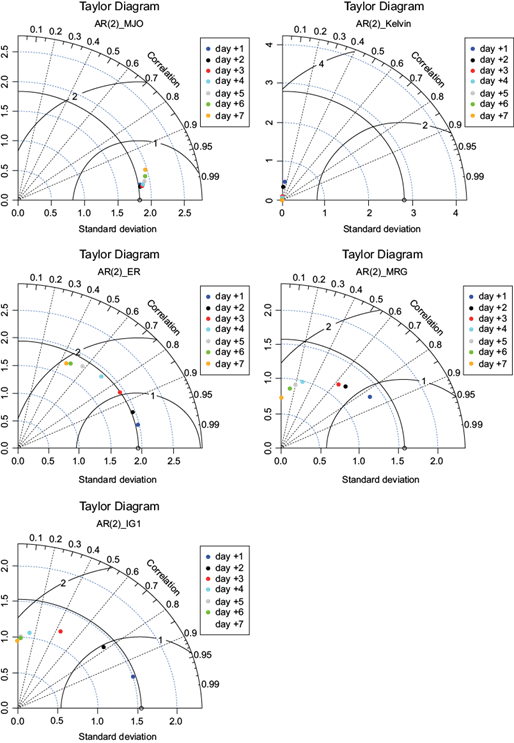
Fig. 6 Taylor diagram of the filtered 3B42-AR(2) for each time lead (dark blue for day +1, black for day +2, red for day +3, cyan for day +4, grey for day +5, light blue for day +6, and orange for day +7) against the filtered 3B42 observations as reference for MJO (upper left), Kelvin (upper right), ER (centre left), MRG (centre right), and IG1 (bottom).
The Taylor diagram for ERA-Interim precipitation forecast calculations in Figure 7 shows a similar value from day +1 through day +7 for all waves, following Figures 4 and 5. Similar to other results, MJO indicates the highest correlation, while IG1 shows the weakest correlation. However, RMSE for all waves shows a slight difference, where IG1 exhibits the lowest RMSE (< 0.17) while ER has the highest (> 0.22), which is also coherent with results in Table II. Meanwhile, the standard deviation shows a quite similar value for all waves except for ER, whch has a closer standard deviation from the reference.
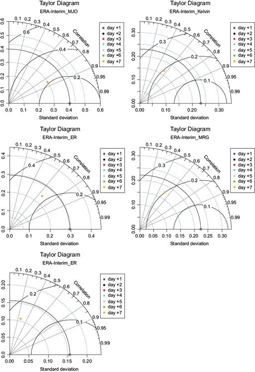
Fig. 7 As in Figure 6, but for the filtered ERA-Interim precipitation forecast process against the filtered 3B42 observation dataset.
From the Taylor diagram, which is also in line with Figures 3 to 5, it becomes clearer that even though the correlation coefficient from the filtered 3B42-AR(2) calculations shows a better result, the error and differences from the reference are higher than the result from ERA-Interim precipitation forecast calculations. Simply put, the wave perturbation pattern forecast for all waves (except Kelvin) is much better for the filtered 3B42-AR(2) calculations. Nevertheless, the wave forecast magnitude shows a better result for ERA-interim precipitation forecast calculation.
4. Conclusion and discussion
The time-series autoregressive forecasting method weighting previous k anomalies associated with k-time, as in Eq. (1), reveals a higher level of accuracy for AR(2) MJO forecasting compared with other waves using correlation coefficient calculation. This is probably caused by the AR(2) calculation being based on previous t-1 and t-2 predictor lag values, for which MJO has a prolonged oscillation period (40-50 days) and a low frequency (Madden and Julian, 1972). On the other hand, the shorter period (< 10 days) of other waves (Kiladis et al., 2009) may cause higher forecast accuracy for MJO at longer forecast leads when compared with other waves (Figs. 3 and 5a). This result is coherent with a previous study which revealed that a strong correlation (> 0.8) was exhibited in the early part (up to day 5) of forecast leads for MJO using a statistical-multivariate lag-regression model, particularly during the southern summer (Jiang et al., 2007). A similar result for MJO forecasts was also achieved by Wheeler and Weickmann (2001) with a strong correlation (of more than 0.8) over the Indonesian region, particularly during the southern summer. This was obtained using an extended frequency-wavenumber spectral analysis derived from the WK99 method. Meanwhile, from the same figures, even though less accuracy is indicated for other waves at longer forecast leads, these are still fairly good until day +2 or +3, probably due to the strong weighted influence of t-1 to t-2 for the AR(2) process. A similar result from the same paper by Wheeler and Weickmann (2001) also revealed that Kelvin waves had a less significant correlation (< 0.4) at day +4, even though more significant than the correlation result exhibited in this study, which is less than 0.1 from the filtered 3B42-AR(2) process. However, this calculation result is less significant compared with the filtered ERA-Interim precipitation forecast process, with correlation lower than 0.6.
The most recent study by Yang et al. (2021) exhibited a higher correlation than the result of this research, that is > 0.6 at least day +4 for Kelvin waves and day +6 for MRG and meridional mode waves number n = 1 and n = 2 ER. Meanwhile, the correlation obtained in this study shows a similar correlation value within day +3 for ER and MRG waves using the filtered 3B42-AR(2) process, and for all forecast times for ER using the filtered ERA-Interim precipitation forecast process. Maybe the references data is one of the causes of this significant difference. Yang et al. (2021) utilized the analysis dataset from the same NWP model as a reference, while this study used a TRMM product as a reference, which is also a proxy of surface precipitation. Another reason is a different reference parameter. Yang et al. (2021) examined wind at 850 hPa, while this study examined a rainfall estimation that includes a complex mechanism compared to other atmospheric parameters. However, both studies suggest that the predictability of the Kelvin wave exhibited a weaker forecast skill compared to other wave types.
The increase in error magnitude calculated by RMSE for the filtered 3B42-AR(2) calculations for day +1 through day +7 (Table I) is presumably caused by the increase in the residual engaged in the next predicted value. This residual increases continuously from the first day of forecast lead to the last, as contained in Eq. (1), particularly for waves with a short period and a high frequency. Compared to other waves, the RMSE residual obtained for MJO is quite small for the filtered 3B42-AR(2) calculation (Table II), probably for the same reason, the prolonged oscillation period of MJO compared with other waves. From the same table it can be seen that the RMSE residuals for the filtered ERA-Interim precipitation forecast calculations are quite small during all forecast leads and for all wave types. This is probably caused by the consistent distribution pattern of the total precipitation-covered area for each different lead time from the ERA-Interim precipitation forecast, even though there is a diverse amount of total precipitation accumulation for each lead time, as already mentioned. RMSE calculation results also correspond to the correlation coefficient, where a consistent correlation for all wave types is exhibited at all forecast lead times. Even though fairly weak at the beginning of the forecast leads compared with the AR(2) results, they do not become negative for the final forecast leads except for IG1. This finding also indicates that the ERA-Interim precipitation model is an adequate for the tropics, especially over Indonesia and associated with the MJO and CCEW forecast models.
Table II As in Table I, but averaged for different forecast leads (i.e., 1 to 7 days) for each wave type.
| MJO | Kelvin | ER | MRG | IG1 | |
| AR(2) | 0.22 | 2.77 | 1.24 | 1.41 | 1.39 |
| ERA | 0.21 | 0.19 | 0.22 | 0.20 | 0.16 |
(AR)2: statistic autoregression method 2; ERA: ERA-Interim reanalysis.
The filtered 3B42-AR(2) forecast shows better wave perturbation patterns for all waves (except Kelvin), but the magnitude of waves shows a better result for the filtered ERA-interim precipitation forecast even though it still cannot be compared to other forecasts. The reason is that previous studies have not been able to assess correlation, RMSE and standard deviation using the Taylor diagram. Thus, this finding becomes a novelty of this study. This finding also corresponds to a previous study which revealed that there is a significant improvement in overall precipitation forecasting accuracy from weather prediction models in the tropics at the present compared with the past decade, particularly for the ERA-Interim forecast model (Janowiak et al. 2010). The most speculative reason mentioned in the same paper is an advancement of cumulus convection schemes which enhances intraseasonal variability in the numerical models. Nevertheless, the discontinuity of ERA-Interim dataset since September 2019 arises a limitation for this paper. The author emphasizes the importance of proposing a similar method for other ongoing datasets to take advantage of this paper's findings.

