


 text new page (beta)
 English (pdf)
 Article in xml format
 Article references
 Send this article by e-mail
 Cited by SciELO
  Similars in
SciELO
Similars in
SciELO 
 Permalink
1. Introduction
We characterize as severe weather the meteorological conditions which potentially may provoke extremely hazardous situations in any aspect of human life. Consequently, for the energy production industry, severe weather is considered as the conditions that may cause extended disruptions to the energy distribution system and, in the worst case, significant interruptions to the energy production and transportation (Zepka et al., 2008). Such impacts may be caused by lightning discharge as well as by severe wind, phenomena closely related to thunderstorms.
Thunderstorms are weather phenomena related to cumulonimbus clouds and develop due to the atmospheric instability on a local or regional scale. They are one of the most spectacular and, simultaneously, dangerous meteorological phenomena, that may be encountered at any time and in any place of the world. Although thunderstorms have a relatively short duration-as an isolated event-they encompass a tremendous power, producing extreme events of lightning strikes, severe winds, heavy precipitation, and hail. All these are potentially dangerous to human life and property (Litta et al., 2013), which is the main reason why meteorologists pay special attention to thunderstorms, trying to understand the mechanisms of their development and to provide forecasts as accurate as possible.
The main factors which especially favor the development and evolution of deep convection are large atmospheric instability and humidity, and the presence of an appropriate lifting mechanism (e.g., Johns and Doswell, 1992; Doswell et al., 1996). In particular, the primary parameters associated with intense, severe, and well-organized local thunderstorms are large convective potential available energy (CAPE) combined with vertical wind shear. Case studies regarding the occurrence of such meteorological conditions in Europe and the USA for the period 1958-1999 are provided by Brooks (2009) and Brooks et al. (2007). As it emerges, the possibility of occurrence of severe phenomena for certain types of weather is higher in the European continent than in the USA, but the specific meteorological conditions that favor this occurrence are rarely encountered. Furthermore, synoptic meteorological conditions combined with local factors, such as complex topography, play an essential role in the initial stage of thunderstorms in Europe. Cases in which meteorological conditions are combined with local factors are examined in many studies (e.g., Schmid et al., 2000; Kaltenböck, 2000a, b, 2004, 2005; Kaltenböck et al., 2004; Dotzek et al., 2001, 2007; Hannesen et al., 1998, 2000; Mazarakis et al., 2008; Galanaki et al., 2015), where the importance of local factors (like orography, inshore areas or areas of convergence, among others) are particularly examined regarding the development and evolution of medium-scale weather phenomena.
Other studies focus on the climatological frequency of severe local wind events and coexisting meteorological conditions (i.e., Wakimoto, 1985; Johns and Hirt, 1987). Although they do not exclusively examine the observed wind gusts produced by thunderstorms, they provide significant information concerning their frequency and the complex thunderstorm environment which result in the development of severe weather conditions (Smith et al., 2013). Furthermore, the literature reveals also studies analyzing the occurrence of severe wind gusts as a result of passing fronts or convective weather with the use of synoptic weather observations as well as data from weather radars (Bartha, 1994). Nevertheless, the knowledge about the special characteristics, climatology and frequency of appearance of such convective gusty winds and their separation from the turbulent gusts, especially in cases of a mixed weather type, is limited.
In this perspective, the forecast of thunderstorms that may produce intense lightning activity accompanied by strong-to-severe wind gusts, for a time horizon of a few hours would be of great importance since it would contribute to the reduction of the negative impacts on, among others, the energy production and distribution sector. Although many efforts have already been devoted in this direction, thunderstorm forecasting remains a particularly challenging topic due to the temporal and spatial extent of such phenomena, combined with the non-linearity of the factors (dynamical and physical) affecting their evolution.
During the last decades many studies were devoted to comprehending the mechanisms that prevail during a thunderstorm event and the way they drive it. Some of these works deal with thunderstorm phenomena and nowcasting (e.g., Schultz et al., 2011; Chaudhuri and Middey, 2013; Wu et al., 2018; Mostajabi et al., 2019), while others tackle the subject of thunderstorm and/or lightning nowcasting (e.g., Rasmussen and Blanchard, 1998; Yair et al., 2010; Kohn et al, 2011; Fierro et al., 2014; Giannaros et al., 2015; Das, 2017; Dafis et al., 2018; Wang et al., 2018). Most of these models are empirical, dynamic or combined. More recent studies using artificial neural networks (ANNs), which are applied to a wide range of applications, have contributed to the improvement of such efforts. These statistical models, which can handle non-linear problems, “learn” the relationship between inputs (independent variables) and outputs (dependent variables) by analyzing past data; they ignore data that do not explain a large part of the variance of the underlying process and concentrate instead on those that do so (Kalogirou, 2001).An important number of ANN application studies can be found in literature (e.g., Kalogirou, 1997; Zhang et al., 1998). These models differ in the network architecture, learning, activation, output functions, etc.
Feng and Kitzmiller (2004)) discuss the set-up and application of an experimental severe weather nowcasting algorithm, based on a back-propagation neural network (BPNN) and compare it with a multiple linear regression model. The BPNN model uses as input weather radar and upper-air data from numerical models. The methods provided essential improvements to the operational Advanced Weather Interactive Processing System (AWIPS) algorithm developed from a much smaller sample of observational data for operational use, while the BPNN approach exhibited higher forecast scores and, overall, a better performance. Zepka et al. (2008)) proposed a cloud-to-ground (CG) lightning forecast system using a back-propagation, multilayer, feed-forward neural network having as inputs lightning data and a number of meteorological (thermodynamic) parameters obtained by the ETA model, which is the operational numerical forecast models run at NCEP, known as the North American Mesoscale (NAM) model. The applied model showed very good results, whose accuracy depends on that of the mesoscale model data and the lightning detection network data used as input. Moreover, Zepka et al. (2014) introduced a lightning forecasting system using neural networks (NN) based on correlations between CG lightning flash data and meteorological variables obtained from MM5 with promising results. In the literature there is a great number of works based on artificial intelligence and data mining techniques (e.g., Sá et al. 2011; Bates et al. 2018; Schön et al., 2019; Mostajabi et al., 2019; Shrestha et al., 2019). An extensive survey of several research papers can be found in Bala et al. (2017)).
In this work we examine the occurrence of extreme wind gusts around a wind power plant, located in a hilly region of western Greece, based on the presence of cumulonimbus clouds and lightning activity. Furthermore, the 1-h forecast of lightning flashes and wind gusts for a horizon of 24 h and with the use of ANN statistical models is analyzed. The examined period spans from January 1, 2012 to December 31, 2014.
The paper is organized as follows: section 2 describes the study area, the wind speed and direction data and the ZEUS network from which we got the lightning activity data; section 2 also explains how a wind gust is determined; section 3 presents the statistical analysis of the observed wind gusts as well as the detected lightning flashes in relation to the meteorological conditions; in section 4 the forecasting procedure is described in detail; section 5 presents the overall forecasting results, and the conclusions are discussed in section 6.
2. Data and methodology
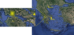
The study focuses on a wind power plant at a hilly area close to the town of Nafpaktos, western Greece, at an altitude between 1000 and 1500 m. The study covers an area between 38º 15’-38º 37’ Ν, and 21º 33’-22º 01’ Ε, a grid box with dimensions 20 × 20 km2 (Fig. 1).
2.1 Wind data
The wind speed and direction are measured at the nacelle of a wind turbine, at a height of 67 magl. Three years of data are used, from January 1, 2012 to December 31, 2014, which consist of the mean wind speed and direction over the last 10 min and the maximum observed wind gust over the same period. These wind data have been aggregated to mean hourly values; the absolute maximum wind gust during the averaging period is also calculated.
The most commonly used approach to determine wind gusts is that of the World Meteorological Organization (WMO), according to which, e.g., the METeorological Aerodrome Report (METAR) and the Aviation SPECIal Weather Report (SPECI), code a wind gust as the maximum horizontal wind speed lasting for at least 3 s if only it exceeds the mean wind speed over the sampling interval by at least 10kts (≈ 5 m s-1) (WMO, 2011a, 2014).
Τhere are also other approaches used on a regional or national level. ΝΟΑΑ (1998) defines the wind gust as the maximum wind speed that lasts 2 s and is 10 kts (≈ 5 m s-1) or higher than the mean wind speed sampled over a 2-min period. In another definition, a gust is the wind speed value lasting for at least 5 s within a 1-h sampling interval (Lombardo et al., 2009; Harris and Kahl, 2017; Letson et al., 2018). According to the WMO (2011b), in Argentina a gust is the maximum hourly average wind speed value that exceeds 30 kts (≈ 15 m s-1). Apart from the difference in the way a wind gust is defined and calculated, it is worth mentioning that there are also numerous approaches concerning the distinction between convective wind gusts and gusts resulting from gradients or local factors (such as topography). De Gaetano et al. (2014) provide a long list of such methods.
In this study we considered as a recorded wind gust the maximum observed wind speed exceeding the average wind speed over the sampling interval by 10 m s-1 (20 kts). The reason for not adhering to the WMO definition is that our data are collected at an altitude of about 1350 m, where the differences between mean wind speed and wind gusts, for any sampling interval, frequently exceed 5.1 m s-1 by far. In fact, the average difference between the hourly mean and the mean maximum wind speed is 5.0 ± 2.0 m s-1 with a maximum of 19.3 m s-1, while the respective average difference by the absolute maximum wind speed is 6.4 ± 2.6 m s-1 with a maximum of 33 m s-1. On the contrary, the proposed limit of 10 m s-1 is observed in fewer cases and mainly when a weather change occurs or is going to occur.
The study focuses on the relationship between wind gusts observed at the wind power plant site and the lightning flashes detected simultaneously inside a specified area (grid box). If one or more wind gusts are recorded at the site of interest, in order to calculate the hourly wind gust values, the data are filtered out to the absolute hourly maximum wind speed and hourly mean wind speed, respectively. Simultaneously an extensive quality control is applied in order to clarify if those wind gusts are due to thunderstorms or to other reasons, e.g., wind speed fluctuations due to local factors such as morphology or even due to possible malfunction of the sensor or the data logger. The data analysis revealed nevertheless that thunderstorms with lightning activity are not always accompanied by gusty winds.
2.2 Lightning data
The required lighting data were provided from the European Network of Lightning Strike Detection ZEUS. This is a large distance network of five receivers placed around Europe with a very good coverage in the central and eastern Mediterranean (Kotroni and Lagouvardos, 2008; Lagouvardos et al., 2009) with a spatial accuracy of the order of 4-5 km. These receivers record the radio signal (sferic) emitted by mainly cloud-to-ground (CG) electric discharges in the VHF range between 7 and 15 kHz. Each receiver captures up to 70 sferics per second; every time such a signal is captured a detection algorithm processes the signal of all the receivers in order to detect the possible sferic candidate, excluding weak signals and noises. Consequently, the location of detected discharge is determined by applying a triangulation technique over the arrival time difference.
It is worth mentioning that the points indicating the occurrence of lightning discharges represent a big portion of the total electric activity, including the IC and CG flashes as well. According also to Maier and Krider (1986)) and Williams et al. (1989), the IC activity prevails in the first stages of the developed thunderstorms, while the CGs occur later.
Drüe et al. (2007) state that the detected discharges are merged and if specific criteria are satisfied then lightning flashes datasets might be created. According to these criteria observed flashes having a spatial difference up to 20 km and a temporal difference of 1 s are considered as one flash. Other studies suggest different approaches. In Cummins et al. (1998) and Diendorfer (2008) the location and time of the first recorded flash consist of an individual lightning datum, while in Piper and Kunz (2017) a day with lightning is considered as when at least five electric discharges are detected in a grid box of 10 ×10 km2.
Because of the apparent difficulty in separating the IC and CG electric discharges, in this study we developed the hourly lightning dataset by processing and clustering the data according to Drüe et al. (2007). So, if a lightning flash fulfils the criteria, the hour of detection is flagged as a flash data independently of the total number of flashes detected during the same period.
3. Statistical analysis of wind gusts and lightning flashes
The frequency of detected lightning discharges over the eastern Mediterranean basin reaches a maximum in autumn (Yair et al., 2010; Kotroni and Lagouvardos, 2016), while most of them occur over maritime and coastal areas rather than overland when warm waters provide the appropriate conditions for storm development. The lightning activity is produced by cumulonimbus clouds due mainly to synoptic scale meteorological conditions (well-organized cyclones) or, in a lesser extent, to passing troughs.
Graeme and Klugmann (2014) demonstrated a clear preference of thunderstorms with lightning activity to occur over land during the warm season of the year. The opposite happens during the cold season, when the majority of these events befall over the sea. The average annual number of electric discharges per km2 in Europe ranges between 0.1 and 4. Galanaki et al. (2015) also studied the cloud-to-ground activity over 10 years (2005-2014) in the eastern Mediterranean basin with similar results. Their results revealed an average annual number of electric discharges between 0.1 and 6, with highest densities over land, while the majority of lightning events over sea befell over the Ionian Sea and the west coastal areas of the Balkans.
The analysis of synoptic charts and thermodynamic diagrams revealed that the general meteorological conditions over our area of interest during 2012-2014 were characterized by a sequence of hot and cold periods accompanied by the corresponding weather phenomena, as normally expected. During winter the development and passage of low-pressure systems results in an important number of lightning flashes, especially over the sea. That type of weather led to a high number of events of severe wind gusts which sometimes lasted for more than two days, as a result of long-lasting frontal activity accompanying those systems. These severe gusts were either related directly to the occurrence of a lightning flash or to the wind profile induced by those pressure systems as the result of the air convection and pressure gradient. As shown in Figure 2, most of the observed wind gusts due or to thunderstorms not, as well as the detected lightning flashes are connected to southern wind directions. The main reason was the frequent passage of well-organized low-pressure systems with extended frontal activity, moving from west to the east and overpassing the area of interest.

Fig. 2 Frequency distribution of wind direction at the wind turbine height related to the total wind gusts (right), wind gusts in the presence of lightnings (middle) and wind gusts in the absence of lighting (left).
The number of lightning flashes and wind gusts within a 1-h period in the site of interest are presented in Table I. The analysis of the dataset of the area of interest for the period from January 1 2012 to December 31, 2014 revealed that a total of 268 lightning strikes occurred, leading to an annual average of 89.3 strikes. The corresponding number of wind gusts, determined according to the definition given in section 2.1, was 937 with an annual average of 312.3 events. The number of wind gusts is divided into those related to lightning strikes and those that are not. From the total of 937 observed wind gusts, 636 (68%) were found to be related to lighting strikes. Nevertheless, only 235 were directly related to the strikes (cases in which a wind gust is observed within the same hour than a lightning strike) while the remaining 401 recorded wind gusts were the result of the general activity of severe weather affecting the surrounding area and producing strong wind gusts sometime before or after the strike. The analysis also revealed that the major portion of the detected lightning strikes (235, 88%) coincided with the observation of strong wind gusts, while the remaining 33 strikes (12%) were not accompanied by gusts or even a slight wind disturbance.
Table I Total number of lightning flashes and wind gusts higher than 10 m s-1 in a period of 1 h. The total number of wind gusts related or not to lightning flashes are also shown.
| Wind gusts | Lightning flashes | Wind gusts related to lightning flashes | Wind gusts not related to lightning flashes |
| 937 | 268 | 636 | 301 |
From Table I it is apparent that 301 of the observed wind gusts (32%) were not related to the occurrence of lightning strikes (direct or indirect) or to any synoptic system. This is attributed to the complex topography of the surrounding area, which combined with specific isobaric situations, might produce severe wind gusts (e.g., high pressure systems from the north combined with low pressure systems from the south, which induce strong north-northeast airstreams or strong southern air flows in the low and middle atmosphere, ahead of a slow moving weather system). Furthermore, a small percentage of such wind gusts is due to recording errors (e.g. instrument’s fault). In that case, the separation of these wind gusts from those due to lightning strikes is practically inevitable.
Figure 3 presents the daily, monthly and seasonal distribution of the total wind gusts and the detected lightning strikes for the examined period. The number of wind gusts related directly or indirectly to lightning strikes and those that are not related are also shown. As shown in the figure, wind gusts and lightning strikes present a maximum in the afternoon and a second peak of smaller magnitude around midnight. It can also be observed that the activity during winter is intense but decreases significantly during the warm period of the year. This is clearly shown in the seasonal distribution, where the recorded wind gusts reach 49% of the cases and lightning strikes 41% of them. These results partially agree with the findings of related studies analyzing the frequency and distribution of detected lightning flashes in the area of interest (Graeme and Klugmann, 2014; Yair et al., 2010). The main reason for this distribution is an intensive frontal activity during the cold period of the year in the area of interest, which has its maximum between December and February. This activity sometimes leads to the development of severe weather frequently accompanied by thunderstorms with intense lighting activity and a strong wind profile (Houze, 2014), especially at the altitude of the wind power plant. These conditions may last for a long period of time (more than two days) (Galanaki et al., 2018).

Fig. 3 Daily (top), monthly (middle) and seasonal (bottom) distribution of total wind gusts (black bars), total lightning strikes (grey bars), wind gusts related to lightning strikes (white bars) and wind gusts not related to lightning strikes (dark grey bars).
Figure 4 emphasizes that the distribution of wind gusts accompanied by lightning strikes is a function of weather types. The different meteorological conditions affecting the surrounding area consist of weather phenomena due to synoptic (e.g., organized cyclones, passing troughs) and atmospheric instability (mainly thermal) conditions. As shown in the figure the wind gusts due to synoptic conditions prevail. These synoptic conditions are more common in Greece during the cold period, i.e., between November and April. As seen in Table II, all wind gusts directly related to lightning strikes were exclusively caused by synoptic weather conditions for most of the months. Of the 199 lightning strikes of this category, 159 (80%) were encountered in this period (between November and April), together with 68% of the total wind gusts directly related to strikes

Fig. 4 Causes of wind gusts (y-axis) related to lightning flashes: synoptic scale (grey bars) and instability (black bars) conditions.
Table II Wind gusts related to flashes vs. weather types.
| Month | Wind gusts related to flashes | Total flashes | Gusts/flashes | Flashes due to instability conditions | Flashes due to synoptic scale conditions |
| January | 127 | 47 | 2.7 | 0 | 47 |
| February | 64 | 19 | 3.4 | 3 | 16 |
| March | 72 | 23 | 3.1 | 2 | 21 |
| April | 59 | 28 | 2.1 | 1 | 27 |
| May | 25 | 10 | 2.5 | 4 | 6 |
| June | 2 | 2 | 1.0 | 2 | 0 |
| July | 7 | 7 | 1.0 | 7 | 0 |
| August | 4 | 4 | 1.0 | 4 | 0 |
| September | 27 | 22 | 1.2 | 6 | 16 |
| October | 54 | 21 | 2.6 | 3 | 18 |
| November | 53 | 22 | 2.4 | 2 | 20 |
| December | 142 | 30 | 4.7 | 2 | 28 |
| Total/average | 636 | 235 | 2.7 | 36 | 199 |
Table II also reveals that 32% of the wind gusts due to synoptic weather types were directly related to lightning strikes. As mentioned earlier, this is because the synoptic weather produces a strong wind profile that expands vertically to the upper atmosphere and also horizontally at large distances ahead of the forthcoming frontal zone (e.g., Houze, 2014). In such cases, wind speed starts increasing as frontal zones approach; eventually, strong wind gusts are recorded even if the lightning flashes in the surrounding area occur later on. Additional evidence that confirms this aspect is shown in Table II (4th column), where the rate of wind gusts per lightning strikes in each month is given, resulting in an annual average equal to 2.7. It is obvious that in most months affected by synoptic weather conditions this rate is high and far from 1, with a maximum in December (4.7), followed by February (3.4) and March (3.1).
On the other hand, when atmospheric instability develops within the study area, weather conditions are characterized by isolated and/or clusters of cumulonimbus clouds, which develop over or close to the mountains and hills, resulting in local showers and thunderstorms sometimes followed by lightning activity, causing intense fluctuations of wind speed and direction. Wind speed increases when these phenomena appear, while the corresponding gusts are produced more or less simultaneously with the lightning flashes. These gusts may be as severe as those of the previous case but of shorter duration, occuring mainly during the presence of isolated thunderstorms and constrained temporally and spatially by the thunderstorm. When thunderstorms dissipate, such wind gusts disappear.
The corresponding percentage of gusts due to isolated thunderstorms directly related to lightning strikes was only 5%. Nevertheless (in contrast to the cases of synoptic weather conditions) in months when instability (mainly thermal) conditions prevail (May to September), the corresponding monthly rate of wind gusts per lightning strikes is too low and (especially during summer) equal to 1 (Table II). This clearly leads to the conclusion that almost all the wind gusts observed during that period of the year and in the area of interest are produced only by isolated thunderstorms mainly over the surrounding hills, and are directly related to the occurrence of lightning strikes.
4. Wind gusts and lightning flashes forecasting
4.1 Thermodynamic parameters
The development of cumulonimbus clouds and thunderstorms is a result of the simultaneous occurrence of a number of factors such as atmospheric instability, large amount of moisture, vertical wind shear and potential available energy (e.g., Johns and Doswell, 1992; Doswell et al., 1996; Rudolf et al., 2010).
In our study, we analyzed the correlation between wind gusts and flashes using four well-known parameters, namely convective available potential energy (CAPE), total totals index (TTI), wind speed at 500 hPa, and the 0 to 6 km vertical wind shear. These parameters are measured using radiosondes or satellites. They can also be obtained from numerical weather prediction models (Davis, 2001). In this study we used data provided by the Copernicus Climate Data Store, generated using Copernicus Climate Change Service (C3S) information (C3S, 2019). The data consist of hourly values with a 0.25º × 0.25º spatial resolution. In what follows we discuss each of the above parameters in detail. We also examine their correlation with flashes and gusts.
4.1.1 Convective potential available energy
The convective potential available energy (CAPE) is one of the main indexes of the possibility of thunderstorms occurrence. CAPE is obtained with Eq. (1):
where LFC is the level of free convection, EL the equilibrium level, θ e the equivalent potential temperature of the air parcel, and θ es the saturated equivalent potential temperature of the atmospheric environment. CAPE stands for positive differences between θ e and θ es , meaning that the pseudo-adiabatic of the displaced air parcel is warmer than that of the environment resulting in instability situations (Sá et al., 2011; Das, 2017). In other words, it is the amount of energy an air-parcel would have in the case it was vertically lifted to a certain height in the atmosphere.
Its value of 250 J kg-1 is a critical limit for the discrimination between thunderstorm and non-thunderstorm classes (Kaltenböck et al., 2009). It is also used to distinguish ordinary thunderstorms from severe events that might cause heavy rain, hail and gusty winds. Figure 5 illustrates the relation between the CAPE and the distribution of the total observed wind speed gusts related and not related to lightning and of the total number of lightning flashes. In this work, it is mainly used to investigate the occurrence of thunderstorms with lightning flashes producing severe wind gusts. In should be noted that the CAPE is mostly connected to instability events not resulting from well-organized cyclones, which are due to local causes such as unstable weather in summer months or the presence of an extended upper low accompanied by cold temperatures. So, in this work the CAPE is not considered as the main representative index for the assessment of lightning activity because (as mentioned in section 3), the lightning flashes are mainly due to frontal weather phenomena and, to a lesser extent, to isolated thunderstorms due to atmospheric instability conditions.
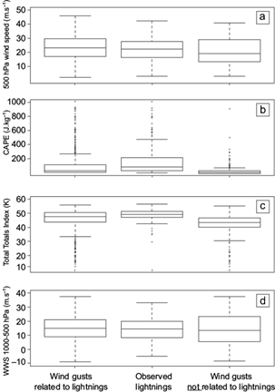
Fig. 5 Box and whisker plots of the total amount of lightning, wind speed gusts related and not related to lightnings, for (a) CAPE, (b) TTI, (c) wind speed at 500 hPa and (d) vertical wind speed between 1000 hPa and 500 hPa. The lower box boundary indicates the 25th percentile, the line within the box the mean, the upper boundary of the box indicates the 75th percentile, while bars above and below the box indicate the 90th and 10th percentiles. The 5% and 95% percentiles are marked as points.
4.1.2 Total totals index
The total totals index (TTI) is an instability index extensively used for a first estimation of thunderstorm events followed by severe weather phenomena, especially in North America (Peppier, 1988). This parameter gives an indication of the probability of occurrence of a thunderstorm and its severity by using the vertical gradient of temperature and humidity. The TTI consists of the arithmetic combination of vertical totals (VT; 850-500 hPa temperature difference) and cross totals (CT; the difference between the 850 hPa dew point and 500 hPa temperature) according to Eq. (2):
The probability of deep convection tends to increase with increasing lapse rate and atmospheric moisture content, while TTI values also vary slightly by geographic location and season. Moreover, 44 K is considered as the value-threshold for the probability of thunderstorms occurrence. Values between 44 and 50 K indicate likely thunderstorms, while values higher than 50 Κ are a strong indication of the development of severe mesoscale convective systems (e.g., Maddox, 1983; Velasco and Fritsch, 1987). Figure 5 presents the relation between the TTI and our parameters of interest. It can be seen that lightning flashes and wind gusts related to them occur preferentially for TTI values around 50 K. It is also shown that when the observed wind gusts are not the result of lightnings the TTI ranges between 40 and 50 K, probably revealing that these gusts are due to other reasons than lightning.
4.1.3 500 hPa wind speed
The 500 hPa isobaric level is particularly important for the evaluation of the atmosphere’s status . Therefore, the wind at that level is a useful parameter for the study of the mid-tropospheric circulation. High wind speeds at 500 hPa are related to severe weather, mainly to gusty winds, because they provide an indication of the downward motion of the developed thunderstorms (Dotzek et al., 2009). In particular the rear-flank downdraft or dry rear inflow of well-organized local thunderstorms is mostly observed when the 500 hPa wind speed is high enough (Kaltenböck, 2004). As shown by the available data, wind speeds of 20 m s-1 or higher constitute a good index of the occurrence of lightning discharges, directly or indirectly accompanied by severe wind gusts (Fig. 5). In cases when wind gusts are not related to thunderstorm presence, the wind speeds at 500 hPa are lower.
4.1.4 0-6 km vertical wind shear
The difference of wind speed between the low (1000 hPa) and upper (500 hPa) atmosphere (vertical wind shear, 0-6 km VWS) is another useful index of imminent atmospheric instability. Higher differences are observed in cases of thunderstorms accompanied with lightning activity and strong wind gusts. When the wind gusts are not due to lightning flashes the VWS values interval is bigger with an average approximately equal to 10 m s-1. On the other hand, more than 50% (between the 25th and 75th percentiles) of the events of lightning discharges and severe wind gusts are related to VWS of about 15 m s-1 (Fig. 5). Therefore, this value is considered as a limit for the discrimination of wind gusts due to lightning those due to other reasons. These findings are in accordance with related works investigating events of severe weather phenomena closely related to thunderstorms and their general activity (e.g., Rasmussen and Blanchard, 1998; Schmid et al., 2000; Kaltenböck et al., 2009).
4.2 Model selection
In this work we propose a multilayer perceptron feed-forward neural network (MLP) model back-propagation learning algorithm in order to predict probable lightning flashes and wind gusts 1 h ahead for a forecasting horizon of 24 h. This type of neural networks are widely applied in various disciplines mainly because they are capable of arbitrary mapping the input-output relationship (Zhang et al., 1995; Wei et al., 2000). Typically, such a network consists of multiple layers of nodes; the first and last layers are the input and the output layers, respectively. Between them there are one or more so-called “hidden” layers of neurons fully interconnected to each other with the use of proper weights. An example of a feed-forward neural network model is presented in Figure 6.

One of the most crucial aspects during an ANN model setup is the selection of the appropriate input values (Alexiadis et al., 1998; Zhang et al., 1998). The model topology, i.e., the number of hidden layers, weights and biases values, the training method, the least acceptable error and the number of iterations during training are the key factors that should be defined in advance, while their optimal combination is heuristic, using a trial-and-error approach. For our purpose we selected feed-forward neural network with a single hidden layer which allows skip-layer connections. As activation function fh of the hidden layer we selected the sigmoid function:
and the linear function as the output layer function, fο. The mοdel οutput y k is given by Eq. (4):
where x i is the inputs, α k and α h are the biases, and w hk and w ih are the set of weights of every link in the network. The sets of weights are adjusted by a general quasi-Newton optimization procedure, the BFGS algorithm (BFGS method), published simultaneously by Broyden (1970)), Fletcher (1970), Goldfarb (1970), and Shanno (1970). This is an iterative algorithm for solving unconstrained non-linear optimization problems. Its advantage is that it gets close to a local minimum reaching it to the machine accuracy after a few iterations (Ripley, 1996). The algorithm uses function values and gradients to build up a picture of the surface to be optimized (Fletcher, 2000) and has been already applied in a variety of works resulting to better model fitting during training that led to more precise forecasts (Liu et al., 2013, 2018).
The inputs of our model are first lags of hourly data of CAPE, TTI, wind speed at 500 hPa and the 0-6 km VWS. Additional inputs tested are the corresponding lags of the difference between mean maximum and mean hourly wind speed as well as the first lag of the absolute maximum wind speed in the same hourly interval. The output layer of our model consists of one neuron providing the 1-h ahead forecast results for the next 24 h, whether or not a wind gust or a flash have been recorded. The output of both neurons is binary, i.e., equal to 0 if no event is forecasted or 1 if an event is forecasted. In order to produce the forecasts, the outputs of the model are parameterized as follows: (i) the “no existence” of the phenomena corresponds to 0; (ii) the “existence” of the phenomena corresponds to 1. Data of a whole year, from January 1, 2012 until December 31, 2012, were used for determining the appropriate model parameters as well as its training. As already mentioned, the activation function is the sigmoid function (Eq. 1) and the linear function as the output function. The error, in order to achieve the optimum model performance is set equal to 10-4, while the maximum number of 1000 to iterations. Table III shows the tested model configurations.
Table III Tested model configurations.
| Model configurations | |||
| Model | Inputs | Network topology | |
| Wind gusts | Flashes | ||
| 1 | Lag-1: absolute maximum wind speed | 1-2-1 | 1-2-1 |
| 2 | Lag-1: absolute maximum wind speed, ΤΤΙ | 2-4-1 | 2-2-1 |
| 3 | Lag-1: absolute maximum wind speed, ΤΤΙ, CAPE | 3-5-1 | 3-4-1 |
| 4 | Lag-1: absolute maximum wind speed, ΤΤΙ, CAPE, 500 hPa wind speed | 4-7-1 | 4-6-1 |
| 5 | Lag-1: absolute maximum wind speed, ΤΤΙ, CAPE, 500 hPa wind speed, 0-6 km VWS | 5-10-1 | 5-7-1 |
| 6 | Lag-1: absolute maximum wind speed, ΤΤΙ, CAPE, 500 hPa wind speed, 0-6 km VWS, mean maximum wind speed-mean wind speed difference | 7-14-1 | 7-12-1 |
| 7 | Lag-1: ΤΤΙ, CAPE, 500 hPa wind speed, 0-6 km VWS | 4-8-1 | 4-6-1 |
VWS: vertical wind shear.
Finally, the overall model performance is evaluated using the root mean square error,
and the mean absolute percentage error,
where N is the number of observations, e t =o t - F t the predicted error, o t the actual observation at time t, and F t the corresponding forecast value. The Pearson correlation coefficient (R2) is also used in order to provide an insight of the model ability to simulate the occurrence of wind gusts and flashes rather than its overall forecasting performance.
5. Results
5.1 Model training
The statistical metrics of the training phase are shown in Table IV. As it can be seen (a) the best forecasts are given by model 6 for the wind gusts and model 5 for flashes, and (b) the training errors decrease each time an additional parameter is used as input. This effect is more pronounced for the wind gust models, the RMSE and MAE, which are finally improved by 52 and 74%, respectively. The corresponding improvement for the flash models is 22 and 29%, respectively. It should also be noted that model configuration 7 using as input the two thermodynamic parameters (CAPE, TTI) as well as wind speed at 500 hPa and the 0-6 km VWS, presents the highest training errors. This could be due either to the uncertainty of these parameters (being the result of reanalysis) or that they provide a more general prediction of future weather conditions, such as the possibility of thunderstorms and their intensity.
Table IV Statistic results of the training phase of the various models.
| Parameter | Applied model | |||||||
| 1 | 2 | 3 | 4 | 5 | 6 | 7 | ||
| Wind gusts | RMSE | 0.13 | 0.11 | 0.12 | 0.11 | 0.1 | 0.063 | 0.14 |
| MAE | 0.034 | 0.027 | 0.029 | 0.026 | 0.026 | 0.009 | 0.044 | |
| R2 | 0.35 | 0.46 | 0.45 | 0.53 | 0.55 | 0.84 | 0.24 | |
| Flashes | RMSE | 0.092 | 0.09 | 0.088 | 0.087 | 0.072 | 0.081 | 0.087 |
| MAE | 0.017 | 0.017 | 0.016 | 0.017 | 0.012 | 0.014 | 0.016 | |
| R2 | 0.06 | 0.11 | 0.13 | 0.15 | 0.43 | 0.28 | 0.16 | |
5.2 Forecast evaluation
In order to test the model effectiveness in forecasting wind gusts and lightning activity in the area of interest, eight time periods, not belonging to the training sample, are used. These periods are expanded from 24 to 72 h and presented in Table V. These periods correspond to three typical meteorological conditions accompanied by a range of weather phenomena and affect the surrounding area during the examined three-year interval (2012-2014). Cases 1 to 3 correspond to well-organized low-pressure systems accompanied by frontal activity. Cases 4 to 6 correspond to thermal instability conditions. Cases 7 and 8 correspond to consecutive passing troughs in the upper (500 hPa) atmosphere.
Table V Forecast cases.
| Case study | Date | Weather conditions |
| 1 | 18/1/2013 | Frontal activity |
| 2 | 24/1/2013 | Frontal activity |
| 3 | 28-29/12/2014 | Frontal activity |
| 4 | 13/5/2013 | Thermal instability |
| 5 | 5/6/2013 | Thermal instability |
| 6 | 8-10/7/2013 | Thermal instability |
| 7 | 27-28/3/2014 | Trough |
| 8 | 23-24/10/2014 | Trough |
The forecasting results for both wind gusts and lightning flashes for the eight selected cases are given in Table VI. It can be seen that wind gust forecasts are more accurate than those of lightning flashes in every case. According to the presented results the model performs better under thermal instability conditions (cases 4 to 6) as well as when gusts of wind are considered as the forecasting parameter. The worst performance was observed for the frontal activity cases (1 to 3).
Table VI Forecasting results of wind gusts and flashes.
| Case study | ||||||||||
| 1 | 2 | 3 | 4 | 5 | 6 | 7 | 8 | Average | ||
| Wind gusts | RMSE | 0.23 | 0.26 | 0.31 | 0.11 | 0.13 | 0.16 | 0.10 | 0.38 | 0.21 |
| MAE | 0.14 | 0.20 | 0.19 | 0.023 | 0.028 | 0.034 | 0.028 | 0.18 | 0.10 | |
| R2 | 0.78 | 0.75 | 0.68 | 0.99 | 0.99 | 0.94 | 0.91 | 0.39 | 0.80 | |
| Lightning flashes | RMSE | 0.50 | 0.53 | 0.34 | 0.20 | 0.21 | 0.20 | 0.24 | 0.36 | 0.32 |
| MAE | 0.35 | 0.36 | 0.14 | 0.048 | 0.049 | 0.048 | 0.090 | 0.15 | 0.15 | |
| R2 | 0.0 | 0.0 | 0.29 | 0.0 | 0.0 | 0.0 | 0.0 | 0.18 | 0.06 | |
Figures 7, 8, 9, 10, 11 and 12 show the forecasting results. As already mentioned, the model forecasts wind gusts with remarkable accuracy. Nevertheless, there is an apparent difference concerning the amplitude of the forecasting curve revealing that the model underestimates future wind gusts. This is probably due to the first phase of forecasts, and especially to input pre-processing and the model training process. On the other hand, lightning flashes forecasts deviate significantly from the real events and are also underestimated, which leads to a worse performance concerning the output flash events for the a few next hours, bigger forecasting errors and, eventually, results of lower credibility and usefulness.

Fig. 7 Forecasted (dashed lines) vs. observed (solid lines) wind gusts (y-axis), for three cases of frontal weather conditions.


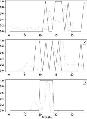
Fig. 10 Forecasted (dashed lines) vs. observed (solid lines) lightning indices (y-axis), for three cases of frontal weather conditions.


The relation between forecasts and the prevailing meteorological conditions at the area of interest needs to be highlighted. When weather phenomena ensued from atmospheric instability, the forecasts of both wind gust and lighting strike events were closer, at least temporally, to the observed data and produce smaller errors. When weather phenomena ensued resulted from well-organized low-pressure systems or were due to a sequence of upper troughs, the forecasted events followed in general the observed ones, but with larger deviations. Again, wind gust forecasts were more accurate compared to those of lightning flashes. A probable cause could be that the number of gusts and flashes occurring during well-organized low-pressure systems differs from that occurring during atmospheric instabilities. When thunderstorms with their lightning activity result from atmospheric instability, the number of observed wind gusts is small and isolated, but when they are due to synoptic weather conditions their number increases significantly. Additionally, in the case of synoptic weather conditions, the phenomena last longer and present important fluctuations during their occurrence, while most of times these phenomena are followed by highly fluctuated gusty wind speeds for a longer period. It should also be noted that the simulated indices and particularly the lightning flashes present significantly lower amplitude compared to those of observations.
6. Discussion and conclusions
In the first part of this study we investigated the relationship between the wind speed gusts recorded at a wind power plant in a hilly area of western Greece and the corresponding lightning strikes detected in the surrounding area for a 3-year (2012-2014) period. The observed wind gusts are strongly correlated with the detected lightning flashes (r = 0.74), both on a seasonal and on a daily basis. Both parameters show a maximum during winter months. On a daily basis, a maximum is observed in the afternoon and a secondary peak during midnight. More than 65% of the overall recorded wind gusts were found to be related directly or indirectly to the presence of cumulonimbus clouds accompanied by lightning activity. On the other hand, the highest percentage of the lightning strikes (almost 90%) detected in the study area was followed by wind gusts and only a small percentage was not accompanied by any change in wind speed or direction.
A major part of the gusty wind patterns affecting the area of interest was found to be due, directly or indirectly, to the development and passage of thunder clouds accompanied by lightning activity. Nevertheless, a percentage of the total amount of the recorded gusts (30-35%) was due to other factors such as strong air streams resulting from the morphology of the area, turbulence in cases of strong upper winds when an atmospheric disturbance approaches without the development of significant weather phenomena, or even the passage over the area of a trough’s edge without causing any weather changes. However, it may be concluded that the presence of certain meteorological conditions that are able to produce severe weather like thunderstorms with lightning activity, causes strong to severe gusty winds. Consequently, those conditions might disrupt the operation of the wind power plant since they may delay or cancel maintenance works, damage the wind turbines or other equipment, or even lead to a complete shutdown in order to protect the wind turbines.
In the second part, we focused on the relation between wind speed gusts and lightning flashes with CAPE, TTI, wind speed at the 500 hPa isobaric level and the 0-6 km vertical wind shear. We also proposed a back-propagation feed forward ANN in order to produce a 1-h ahead forecast of these two variables. The proposed model manages to simulate the variability of the occurrence both of wind gusts and lightning flashes, especially when the four selected parameters were combined with wind data coming directly from wind turbines, such as absolute maximum and mean wind speeds. The forecasted wind speed gust values were more accurate and presented smaller errors, compared to those of flashes, which were underestimated. Nevertheless, despite the apparent underestimations the model manages to capture the fluctuation of wind gusts and, in a smaller extent, of flashes occurrence. Based on these conclusions, we state that our model might provide good 1-h ahead forecasts of the wind speed gusts for a forecasting horizon of 1 to 72 h beforehand. Also, in the case of lightning flashes the proposed method may lead to a good evidence of the possibility of occurrence of such events, although such predictions still need great advances in scientific knowledge.
Lightning flashes are characterized by important spatial and temporal variability. Therefore, the performance of the proposed model is expected to be further improved if data of higher spatial and temporal resolution are available. In addition, we suggest combining the output of our model with those of high-resolution numerical models covering a longer time period and a larger area, in order to improve accuracy. Also, understanding the significance of local and medium scale factors during the development and evolution of severe phenomena is a key parameter. In this context, data from other sites might also give additional insight of the way in which weather phenomena produce severe events. Such an analysis needs to be precisely designed in advance and include both coastal and mountainous areas as well as their combination, according to their special wind and temperature profile (Rudolf et al., 2010). This type of analysis would be very useful, especially for areas like Greece, characterized by a complex morphology and abrupt terrain variations and changes between land and sea, where many sites could be potentially used for the construction of wind power plants.

