


 text new page (beta)
 English (pdf)
 Article in xml format
 Article references
 Send this article by e-mail
 Cited by SciELO
  Similars in
SciELO
Similars in
SciELO 
 Permalink
1. Introduction
Northeastern Brazil experiences a semiarid climatic regime, and over 80% of the area often decrees a state of public emergency due to extreme drought. However, most of the population lives along the coast, where the rainfall regime can occur intensely or depend on several ocean-atmosphere processes, or a combination of these factors (Kouadio et al., 2012). The occurrence of heavy rain and storms in the region typically causes flash floods, power outages, damage to road structures, and material and human losses; therefore, these extreme weather events are highly disruptive to the urban system and pose a major challenge to the government and society.
Some adaptive measures have been implemented to prevent and mitigate these weather conditions, and convection-permitting models (CPM) have been appropriate to characterize extreme rainfall events. Forecasting centers have successfully improved the precision in representing this severe weather environment using CPM, however, computational costs to implement these models are higher compared to numerical weather prediction (NWP) models that use parameterization schemes to represent convection (Clark et al., 2016; Chan et al., 2018; Woodhams et al., 2018). Even though, accurately representing any extreme weather event with realistic temporal and spatial distribution remains a challenge in NWP studies, particularly over coastal and tropical areas with intense convective characteristics that can change rapidly due to the influences of land-sea breezes and mesoscale systems (Hariprasad et al., 2014; Salvador et al., 2016; Surussavadee, 2017). The Center for Weather Forecasts and Climate Studies of the Brazilian National Institute for Space Research (CPTEC/INPE) provides information regarding weather conditions by employing a modeling domain that covers South America (Chou et al., 2005, 2014; Solman et al., 2013). However, global and hemispheric models cannot represent the local to regional characteristics of the spatiotemporal variability of precipitation; therefore, regional models are preferable for properly representing physical processes. As such, local information could be more valuable to local urban planners for managing more efficient solutions. Doppler Weather Radar (DWR) data are a vital source of information for studying the characteristics of mesoscale systems (Gao et al., 1999; Kim and Lee, 2006, but the lack of adequate observational data has prompted numerous researchers to apply mesoscale numerical models for identifying the mesoscale features and studying the evolution and propagation of extreme rainfall. Furthermore, the present heavy precipitation prediction capabilities are limited due to the uncertainties in the initial state, coarse resolution, and physics parameterization techniques of the model (Bei and Zhang, 2007; Hally et al., 2014).
The mesoscale numerical Weather Research and Forecasting (WRF) model, which is an advanced atmospheric model, allows users to select physics and dynamics settings that can be more suitable for a given region, and has gained wider popularity due to its various applications that aid the performance of numerical experiments, allowing a better understanding of the atmospheric dynamics of some episodes or phenomena such as precipitation, heat and cold events, pollution, wind cycles, and severe storms. However, some physical processes cannot be described by traditional fluid mechanics equations; therefore, several researchers have undertaken the development of a parameterization that can effectively describe the spatial and temporal evolutions of these processes (Chen et al., 1996; Koren et al., 1999; Chen and Dudhia, 2001; Salvador et al., 2016). It is widely agreed that the best model configuration will depend on the studied area and time of the year, and relevant research has been mainly conducted in tropical and mid-high latitudes (Jiménez et al., 2006; Balzarini et al., 2014; Carvalho et al., 2014; Ekström, 2015; Banks et al., 2016; Sharma et al., 2016; Avolio et al., 2017; Powers et al., 2017; Imran et al., 2018; Lian et al., 2018; Tymvios et al., 2018), with few studies conducted in tropical and coastal regions or lower latitudes (Hariprasad et al., 2014; Boadh et al., 2016; Gunwani and Mohan, 2017; Penchah et al., 2017).
Salvador city, the capital of the state of Bahia, Brazil, experiences the highest number of natural disasters associated with intense rain on the coast of the northeast region of the country, and rainfall is mostly concentrated between April and July (Rao et al., 1993). The occurrence of intense rain is very rare outside this period. However, the Guará cyclone/subtropical storm occurred on December 9, 2017, originating from a strong decrease in atmospheric pressure between the coast of southern Bahia and northern Espírito Santo state. The cyclone caused strong winds that devastated several areas of the city, and waves of up to 5 m, according to the Brazilian Navy. Therefore, to analyze this event in the metropolitan region of Salvador (MRS), 63 runs using different combinations of seven microphysics (MP), three cumulus (CU), and three planetary boundary layer (PBL) schemes with a very fine resolution (1 km) were conducted to elucidate the most suitable physical parameterization scheme for this extreme rainfall event over an urban-coastal area. This extreme rainfall event was selected since it can be difficult for the model to depict such abrupt changes in atmospheric behavior (Surussavadee, 2017). Therefore, this case study was conducted to evaluate parameterizations in a coastal region during extreme rainfall by comparing the modeled results with data obtained at meteorological stations. Few studies have evaluated the parameterizations used in the WRF model under extreme rainfall conditions over coastal regions, even though the coastal zone of Brazil extends for over 8500 km.
The remainder of this paper is organized as follows. Section 2 presents the methodology, with a description of the meteorological event, WRF physical parameterization schemes, and statistical indices used in the evaluation of the model performance. Section 3 presents and compares the numerical results to experimental data. Finally, the conclusions are presented in section 4.
2. Methodology
2.1 Description of the observed meteorological event
The MRS, which is an urban-industrial and coastal area formed by 13 cities with a total population of over four million inhabitants, was affected by a subtropical storm, Guará, on December 9, 2017. During this event, 23.6 mm of precipitation were measured within 1 h (between 17:00 and 18:00 LT) at the Brazilian National Institute of Meteorology (INMET) meteorological station located in Salvador (Fig. 1), the largest city and capital of Bahia state. The hottest day of 2017 was also recorded on the same day (34.9 ºC) at INMET and International Airport stations. The high temperatures associated with humidity originating from the Amazon region and ocean intensified the cloudiness, and heavy rain with lightning struck the region. According to the Brazilian Navy Hydrography Center, a frontal system moved from the Atlantic Ocean (east) to the MRS (west), with a minimum atmospheric pressure of 998 hPa and wind speed of 74 km h-1 (~ 20 m s-1), which caused strong wind fields and rainfall over the MRS. The South Atlantic Convergence Zone (SACZ) exerts its greatest influence over Brazil during the end of spring and summer, and can extend from the Amazon basin to the subtropical Atlantic Ocean, provoking rainfall over the north, central-west, and southeast regions (Carvalho et al., 2004). During the analyzed episode, the synoptic weather charts indicated the presence of SACZ over 15 consecutive days, and mainly acted over the midwest-southeast and northeast Brazil, where the presence of the SACZ is considered anomalous.

2.2 WRF physical parameterization schemes and modeling setup
Moisture, heat, and momentum exchange within the planetary boundary layer through mixing associated with turbulent eddies that influence the evolution of lower-tropospheric thermodynamic and kinematic structures. However, such eddies operate on spatiotemporal scales that cannot be explicitly represented on the grid scales and time steps employed in most NWP models. Therefore, their effects are expressed through mathematical equations, which are also called physical parameterization schemes (Stensrud, 2007). The conventional parameterizations in the WRF model include the longwave and shortwave radiation, PBL, surface layer (SL), cumulus (CU), and microphysics (MP) schemes.
The MP parameterization scheme controls the various types of precipitation processes and humidity by modifying the air temperature based on the interaction between clouds and radiation, and the absorption and latent heat release due to the phase changes of water. The impact of MP schemes on the subtropical storm Guará was examined using seven MP options in the WRF model: Kessler, Lin, WRF single-moment 3 (WSM3), WRF single-moment 5 (WSM5), WRF single-moment 6 (WSM6), Eta and Goddard schemes. They are categorized as bulk schemes, and usually represent the size distributions of particles, referred as hydrometeors species, through gamma distribution functions that use the mixing ratio and/or the number concentration (Li et al., 2008; Comin et al., 2018; Lee and Baik, 2018). Thus, one of the major differences between the MP schemes is related to the number of hydrometeors considered as prognostic variable, namely: water vapor (v), cloud droplets (c), rainwater (r), cloud ice (i), snow (s), and graupel (g). Kessler is a simple warm cloud scheme that considers v, c, and r classes. The others are mixed-phase schemes that evolved from Kessler and are considered more sophisticated because more numbers of hydrometeors are used (Skamarock et al., 2008). However, sophisticated schemes are not synonym of meaningful improvements, that is why it is recommended to perform an evaluation to establish the cost benefit of longer simulations and computational expense due to the use of more sophisticated schemes (Jeworrek et al., 2019).
The CU schemes are responsible for the sub-grid effects of convective and/or shallow clouds as a consequence of larger-scale processes. Thus, these schemes are responsible for the distribution of moisture and heat that influence clouds formation and precipitation prediction. Theoretically, CU schemes are not activated for fine grid sizes, because it is assumed that regional models are able to resolve organized convection. Thus, in the present work, Kain-Fritsch (KF), Betts-Miller-Janjić (BMJ) and Grell-Freitas (GF) schemes were only activated on the coarsest grid (D01) and switched off on the finer grids (D02 and D03). KF and GF are mass flux parameterizations, from which the former has been widely used by operational applications (Zheng et al., 2016). It is based on the early version of KF, that used a relatively simple cloud model (Skamarock et al., 2008). The latter is based on the Grell-Devenyi scheme, and was formulated to be used in high resolution mesoscale models. It was developed through experiments over South America, using the Brazilian version of the Regional Atmospheric Modeling system (BRAMS) (Grell and Freitas, 2014), which could be more realistic for our study. BMJ scheme is an adjustment type scheme that uses reference profiles from a field campaign at the tropical Atlantic Ocean from Africa to South America in 1974, to adjust vertical profile of temperature and humidity (Janjić, 2000).
The PBL parameterization schemes represent the vertical sub-grid scale fluxes, known as eddies, due to turbulence that can be generated by buoyancy or shear throughout the entire grid column, and not just in the boundary layer. The treatment of the moisture, heat, and momentum exchange processes in the PBL by the WRF considers the order of turbulence closure and whether the employed mixing approach is local or non-local. Among the three PBL schemes evaluated in this study, the Yonsei University (YSU) is a first-order non-local scheme that uses information of multiple vertical levels to determine a variable at a given point. The non-local vertical fluxes are reached by adding a non-local gradient adjustment term to the local gradient for any prognostic variables (Hong et al., 2006). The non-local approach has been suggested to be better because they would be able to account the amount of turbulence generated by large vortices, as opposed to the local closure schemes, which only use the variables of vertical levels that are directly adjacent to the given point. To overcome this deficiency, higher orders of treatments have been developed (Mellor and Yamada, 1982), such as the Mellor-Yamada-Janjić (MYJ) scheme, which is one-and-a-half order local closure. The Asymmetric Convective Model 2 (ACM2) considers both approaches depending on the stability conditions, which hypothetical would be an ideal scheme (Kolling et al., 2013). Like YSU, ACM2 has an eddy diffusion component in addition to the explicit nonlocal transport. The SL schemes calculate the friction velocities and exchange coefficients used in the calculation of surface heat and moisture fluxes by the land surface models and surface stress in the PBL schemes. As some PBL schemes are tied to a unique SL scheme, three SL schemes were used in the simulations: Eta to MYJ, MM5 to YSU, and PX to ACM2 (Skamarock et al., 2008).
As the simulations were conducted for an extreme rainfall event, this work considered combinations of different PBL, CU, and MP schemes. The selection of the MP scheme influences the spatial pattern of rainfall, while the selection of the PBL and CU parameterization schemes influences the magnitude of rainfall in the WRF model during extreme rainfall events (Chawla et al., 2018; Singh et al., 2018, Song and Sohn, 2018). The non-local PBL closure schemes simulate heavy rainfall events more correctly close to the sea, while other configurations more accurately predict rainfall in mountainous terrains (Avolio and Federico, 2018). Although no scheme uniformly represents well all atmospheric conditions (Shin et al., 2012), the most suitable physical parameterization ensemble that represents the atmosphere dynamics over a region must be elucidated. Therefore, 63 simulations using different combinations of MP, CU, and PBL schemes were evaluated based on their ability to simulate hourly precipitation during the extreme rainfall event. The physical parameterization schemes were selected based on whether they directly influenced the representation of precipitation production by the model. As no previous studies had assessed the MRS using the WRF model, the most common parameterization schemes found in literature were tested. Furthermore, the study was conducted using version 3.9 of the WRF model with the Advanced Research WRF (ARW) dynamical solver. The meteorological data were obtained from NCEP Final Analysis (FNL) with a grid resolution of 0.25 × 0.25º every 6 h (NCEP, 2015). The MODIS land-use dataset was used, which is the default land-use dataset of the WRF. The simulations were set to run from December 5 to 10, 2017. The model was run with three nested domains and grid resolutions of 9 km (D01), 3 km (D02), and 1 km (D03; see Fig. 1). The domain of interest (D03) had a horizontal resolution of 1 km and 23 vertical levels with the model top set to 50 hPa. An overview of the physical and spatial configuration of WRF is shown in Table I. The references of each option available in the WRF model can be found in its manual and in Skamarock et al. (2008).
Table I Details of the physical parameterization schemes and spatial configuration adopted in the WRF simulations.
| Domain | D01 | D02 | D03 |
| Horizontal resolution | 9 km | 3 km | 1 km |
| Domain cell numbers | 39 × 39 × 23 | 60 × 60 × 23 | 132 × 132 × 23 |
| Domain size | 11.18º-14.33º S 36.66º-39.92º W 359 × 359 km | 11.99º-13.61º S 37.58º-39.25º W 180 × 180 km | 12.18º-13.37º S 37.78º-39.00º W 132 × 132 km |
| Longwave radiation | Dudhia scheme (option 1) | ||
| Shortwave radiation | Rapid Radiative Transfer Model (option 1) | ||
| Land surface scheme | Noah land-surface model (option 1) | ||
| Microphysics (MP) | Kessler (option 1) Lin (option 2) WRF single-moment 3 (WSM3) (option 3) WRF single-moment 5 (WSM5) (option 4) WRF single-moment 6 (WSM6) (option 6) Eta scheme (option 4 Goddard (option 7) | ||
| Cumulus (CU) | Kain-Fritsch (KF) (option 1) Betts-Miller-Janjić (BMJ) (option 2) Grell-Freitas (GF) (option 3) | ||
| Planetary boundary layer (PBL) | Mellor-Yamada-Janjić (MYJ) (option 2) Yonsei University (YSU) (option 1) Asymmetric Convective Model 2 (ACM2) (option 7) | ||
| Surface layer (SL) | Eta similarity (option 2) MM5 (option 1) Pleim-Xiu (PX) (option 7) | ||
2.3 Evaluation of the model performance
The model performance was evaluated by comparing the hourly observed and modeled data. The latter was extracted from the grid point nearest to the latitude and longitude of the ground weather stations in D03, whose locations are displayed in Fig. 1. These were INMET (13.01 ºS, 38.52 ºW, 51.41 m above the ground) and the Airport (12.91 ºS, 38.33 ºW, 19.51 m above the ground). The former is represented by the following observed meteorological parameters: wind speed at 10 m (WS10), wind direction at 10 m (WD10), temperature at 2 m (T2), relative humidity at 2 m (RH2), and precipitation (RAIN).
The following statistical indices recommended by Zhang et al. (2012) and Emery et al. (2001) were computed: mean bias (MB), standard deviation of the modeled data (SD), root-mean-square-error (RMSE), mean absolute gross error (MAGE), correlation coefficient (R), index of agreement (IOA), and the fraction of predictions within a factor of two observations (FAC2). The MB, RMSE, and MAGE are indices related to the errors and deviations of the model. Therefore, high-quality simulations have values closer to zero. R, IOA, and FAC2 are indices of association and agreement between modeled and observed data, with zero indicating an absence of correlation and values closer to 1 indicating a strong correlation. As wind direction is a circular variable, the errors should be calculated considering the shortest angular distance between the modeled and observed data (Jiménez and Dudhia, 2013). Therefore, for wind direction, if the observed or modeled value was greater than 180º, 360 was subtracted.
The indices are presented as Taylor diagrams (Taylor, 2001) and soccer plots in the following section. The different markers and colors represented the 63 simulations. The numbers in the Taylor diagrams represent the combination of the PBL and CU schemes, while the colors represent the different MP schemes, with 01, 02, 03, 04, 05, 06, 07, 08, and 09 indicating MYJ-KF, MYJ-BMJ, MYJ-GF, YSU-KF, YSU-BMJ, YSU-GF, ACM2-KF, ACM2-BMJ, and ACM2-GF, respectively. In addition, the best configuration is identified through a scoring procedure, following Somos-Valenzuela and Manquehual-Cheuque (2020). The configuration with the best score receives a value of 1, adding a unit to the next, while the worst score receives a value of 63. This procedure is repeated for each station and parameter. Finally, the score is summed, and the configuration with the lowest value is the one with the best performance for the variable.
3. Numerical results
The results of the simulations conducted with the WRF model during the passing subtropical storm Guará are presented to elucidate whether the mesoscale model could capture this extreme rainfall event. The performance of the parameterization schemes considering wind speed, wind direction, temperature, relative humidity, and rainfall is first presented, followed by the spatial distribution of the wind fields and precipitation.
3.1 Parameterization schemes performance
3.1.1 Wind speed results
Figure 2 shows the comparison soccer plot for the RMSE and MB statistical metrics of WS10 from the INMET and Airport meteorological stations.
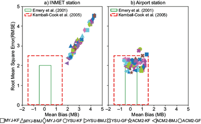
Fig. 2 Comparison soccer plot for the statistical metrics of RMSE and MB for WS10. The green line represents the statistical benchmarks suggested by Emery et al. (2001) for WS10 over simple terrains (MB ≤ ±0.5 m s-1 and RMSE ≤ 2 m s-1), while the red line represents the statistical benchmarks suggested by Kemball-Cook et al. (2005) over complex terrains (MB ≤ ± 1.5 m s-1 and RMSE ≤ 2.5 m s-1).
The very low wind speed values registered at the INMET ground station were due to the presence of vegetation and hills surrounding the station. Over built areas, the presence of obstructions slows down the wind speed, and besides the WRF model was formulated for mesoscale systems. To have a better agreement with observed wind speed over built areas, it is suggested to turn on the urban physics schemes that use lower values for land surface parameters (Martilli et al., 2002; Sarmiento et al., 2017). Therefore, by comparing the WRF results with the INMET data (Fig. 2a), the statistical error indices (RMSE and MB) did not agree well, and all runs were overestimated.
Figure 3 shows the WS10 comparison Taylor diagram for the SD (blue line) and R (black line) statistical metrics. The highest positive correlation (R = 0.68) was obtained for the MYJ-KF-Eta configuration (ID 01, pink marker), while the most negative correlation (R = -0.73) was obtained for the MYJ-BMJ-WSM6 ensemble (ID 02, purple marker) for the INMET station. The IOA and FAC2 did not exceed 0.60 and 0.50 for any simulation, as suggested by Emery et al. (2001) and Hanna and Chang (2012), respectively, as these are conservative benchmarks that consider analyses over simple terrains and rural areas.
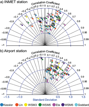
Fig. 3 WS10 comparison Taylor diagram for the SD (blue line) and R (black line) statistical metrics. (a) INMET and (b) Airport stations. The numbers 01, 02, 03, 04, 05, 06, 07, 08, and 09 indicate MYJ-KF, MYJ-BMJ, MYJ-GF, YSU-KF, YSU-BMJ, YSU-GF, ACM2-KF, ACM2-BMJ, and ACM2-GF, respectively
The best statistical indices for WS10 were related to the Airport station, where the different combination schemes exhibited similar deviations. However, the simulations using the ACM2-PBL scheme (regardless of the type of CU parameterization used) exhibited the smallest deviations for both stations (Fig. 2).
The Taylor diagram (in Fig. 3b) indicates there were significant differences between the results. The simulations using the MYJ-PBL scheme with KF (ID 01) and GD (ID 03) had the highest R values for WS10, with the best scores achieved by the MYJ-KF-Kessler (R = 0.76, IOA = 0.74, FAC2 = 0.75), MYJ-KF-WSM6 (R = 0.75, IOA = 0.75, FAC2 = 0.83) and MYJ-GF-Lin (R = 0.72, IOA = 0.72, FAC2 = 0.71) configurations. Additionally, all simulations using the YSU-PBL scheme, and most simulations with ACM2-PBL scheme did not achieve an IOA value of over 0.60, regardless of the CU and MP schemes.
3.1.2 Wind direction results
Figure 4 shows a comparison soccer plot for the MAGE and MB statistical metrics at the INMET and Airport meteorological stations for WD10. The observed WD10 values were more similar between both stations, with most winds originating from the north, northeast, and northwest directions. According to the WRF results, the majority of simulated wind direction had a positive bias (clockwise) during the period, with a mean error varying between 0º and 20º. The lowest deviations were obtained for the MYJ-GF-Lin configuration for INMET station (brown diamond in Fig. 4a), and MYJ-GF (diamond markers in Fig. 4b), regardless of the MP parameterization used for the Airport station. Emery et al. (2001) indicate that the MB and MAGE of WD10 should be less than ± 10º and 30º, respectively, while Kemball-Cook et al. (2005) stated that MAGE should be below 55º over complex terrains.
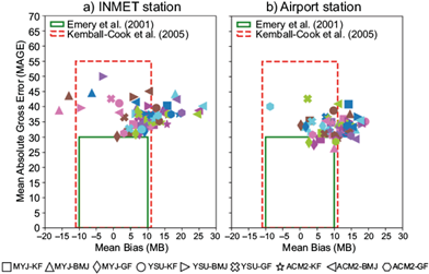
Fig. 4 WD10 comparison soccer plot for the MAGE and MB statistical metrics. The green line represents the statistical benchmarks suggested by Emery et al. (2001) for WD10 over simple terrain (MB ≤ ±10º and MAGE ≤ 30º), and the red line represents the statistical benchmarks suggested by Kemball-Cook et al. (2005) over complex terrain (MAGE ≤ 55º).
The largest amount of FAC2 values greater than 0.5 for INMET station were achieved for the simulations using the GF-CU scheme, even though a single configuration was emphasized for the Airport station. The highest IOA values were associated with MYJ-KF-Lin (IOA = 0.67) for the INMET station, and YSU-GF-Kessler (IOA = 0.70) for the Airport station.
Figure 5 shows the WD10 comparison Taylor diagram for the SD (blue line) and R (black line) statistical metrics at the INMET and Airport meteorological stations.
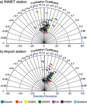
Fig. 5 WD10 comparison Taylor diagram for the SD (blue line) and R (black line) statistical metrics. (a) INMET and (b) Airport stations. The numbers 01, 02, 03, 04, 05, 06, 07, 08, and 09 represent MYJ-KF, MYJ-BMJ, MYJ-GF, YSU-KF, YSU-BMJ, YSU-GF, ACM2-KF, ACM2-BMJ, and ACM2-GF, respectively.
The R-values were very low as the analysis of this parameter is critical due to the sudden change in wind direction. The highest correlation values were achieved for the MYJ-KF-Lin (ID 01, orange marker; R = 0.48) and ACM2-BMJ-WSM3 (ID 08, yellow marker; R = 0.60) configurations for the INMET (Fig. 5a) and Airport (Fig. 5b) stations, respectively. Both configurations also exhibited reasonable agreement indices (MYJ-KF-Lin: IOA = 0.67, FAC2 = 0.46; ACM2-BMJ-WSM3: IOA = 0.63, FAC2 = 0.42).
3.1.3 Temperature and relative humidity
Figure 6 shows an hourly comparison of T2 between observed and modeled data at the INMET station on December 9, 2017, which was the hottest day in 2017 registered in the region, with a thermal amplitude of 11.8 ºC. This great variation could be challenging for the model to emulate, even though most of the simulations could depict this oscillation (Fig. 6).
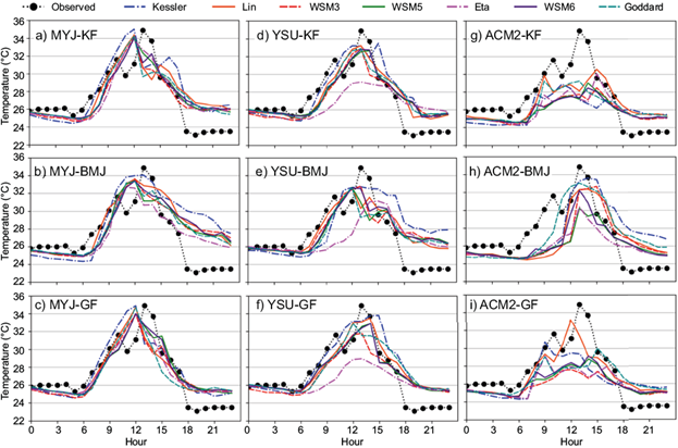
Fig. 6 Time-series of T2 from the INMET data (observed) and numerical simulations of Subtropical Storm Guará over MRS on December 9, 2017, with different MP, PBL, and CU schemes
Statistical indices showed that the mean errors were acceptable, with most of the simulations meeting the criteria suggested by Emery et al. (2001), which are more conservative than those suggested by Kemball-Cook et al. (2005). Additionally, IOA and FAC2 values of ≥ 0.80 and ≥ 0.50 are also recommended, respectively, which were met by most simulations, excluding the BMJ CU and ACM2 PBL schemes. The combination of both schemes (ACM2 + BMJ) achieved the worst R and IOA values for T2. The results of T2 were very uniform for MYJ-PBL and YSU-PBL (except using Eta-MP), which also produced the smallest deviations and highest agreement index values, together with the GF-CU scheme.
Figure 7 shows the T2 comparison Taylor diagram for the SD (blue line) and R (black line) statistical metrics at the INMET and Airport meteorological stations.
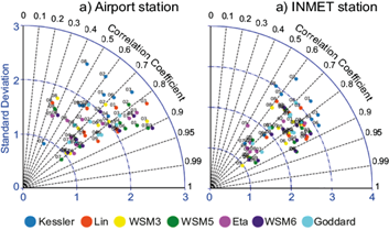
Fig. 7 T2 comparison Taylor diagram for the SD (blue line) and R (black line) statistical metrics. (a) INMET and (b) Airport stations. The numbers 01, 02, 03, 04, 05, 06, 07, 08, and 09 represent MYJ-KF, MYJ-BMJ, MYJ-GF, YSU-KF, YSU-BMJ, YSU-GF, ACM2-KF, ACM2-BMJ, and ACM2-GF, respectively.
The highest correlation values were achieved by the YSU-GF-WSM5 (R = 0.92, IOA = 0.93, FAC2 = 1.00) and MYJ-GF-WSM6 (R = 0.91, IOA = 0.95, FAC2 = 1.00) for the INMET and Airport stations (ID 06-03, purple and green markers in Figs 7a-b). Therefore, the GF-CU scheme with the MP-WSM series is a suitable combination of physical parameterization schemes in the WRF model for studies that mainly aim to evaluate temperature, such as those assessing the urban heat island effects.
Figure 8 shows the RH2 comparison soccer plot and Taylor diagram for the MAGE, MB, SD, and R statistical metrics at the INMET meteorological station.
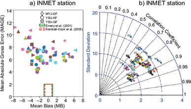
Fig. 8 RH2 comparison soccer plot (a) and Taylor diagram (b) for the MAGE, MB, SD, and R statistical metrics at the INMET station. The green line represents the statistical benchmarks suggested by Emery et al. (2001) for RH2 over simple terrain (MB ≤ ±1 g kg-1 and MAGE ≤ 2 g kg-1), and the red line represents the statistical benchmarks suggested by Kemball-Cook et al. (2005) over complex terrain (MB ≤ ± 0.80 g kg-1 and MAGE ≤ 2 g kg-1).
RH2 data were only available at the INMET station, where the relative humidity varied between 47 and 93%, with an average of 75%. None of the simulations met the error benchmarks recommended by Emery et al. (2001) and Kemball-Cook et al. (2005) (Fig. 8a). In contrast, all simulations met FAC2 ≥ 0.50 and IOA ≥ 0.60. The lowest deviations were achieved by the simulations that used the YSU-PBL scheme with the KF and GF-CU schemes (ID 04-06 with orange [Lin], green [WSM5], and purple [WSM6] markers in Fig. 8b). Therefore, despite the moderate deviations, the values of the agreement indices were high, with the best score achieved by YSU-GF-WSM6 (R = 0.93, IOA = 0.96, FAC2 = 1.00) due to the good results achieved for T2.
Table II shows the configuration of PBL, MP, and CU schemes that were highlighted considering the statistical indices for WS10, WD10, T2 and RH2 and each station. The scoring procedure was used for the selection of each configuration. The MYJ-PBL and GF-CU schemes could be reasonable for evaluations related to wind direction and relative humidity, whereas the YSU- PBL and WSM6-MP schemes for temperature.
3.1.4 Rainfall results
In the WRF model, rainfall is based on two variables: RAINC and RAINNC, which are the rainfall produced by cumulus parameterization and grid-scale processes, respectively. Therefore, the total rainfall would be the sum of the variables RAINC and RAINNC. However, as the cumulus parameterization was switched off under D02 and D03, the sole contributor to the total rainfall under these domains was the variable RAINNC. Additionally, the hourly precipitation has to be subtracted from the previous hour because both are cumulative variables.
Figure 9 shows the time-series of RAIN from INMET data (observed) and numerical simulations of subtropical storm Guará over MRS on December 9, 2017 with different MP, PBL, and CU schemes using data from D03 (the domain of interest). The rain gauge at INMET station registered 23.6 mm of rainfall within 1 h (between 17:00-18:00 LT), and accumulated daily precipitation of 40.80 mm.
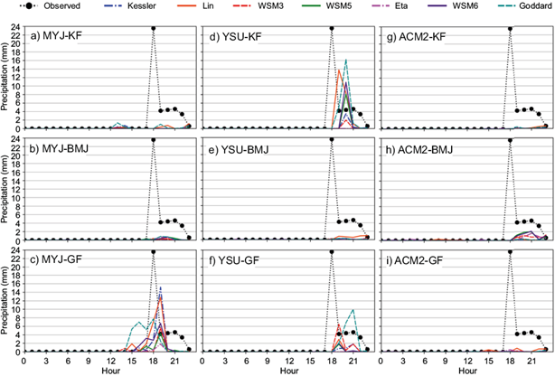
Fig. 9 Time-series of RAIN from the INMET data (observed) and numerical simulations of subtropical storm Guará over MRS on December 9, 2017, with different MP, PBL, and CU schemes.
The MYJ-GF, YSU-KF, and YSU-GF schemes (depending on the MP scheme adopted) were able to simulate the precipitation peaks with time lags and quantitative errors (Fig. 9c, d, f).
The MYJ-GF-Goddard, with a value of 7.7 mm, and MYJ-GF-Lin, with a value of 7.1 mm, produced reasonable rainfall values at the same time as the storm. However, the MYJ-GF-Goddard configuration reported the occurrence of rainfall 3 h before the event. The other MYJ-GF ensembles (Fig. 9c) depicted the storm with a time lag of 1 h, and their results decreased in the following order MYJ-GF-Kessler (15.2 mm) and MYJ-GF-Lin (12.8 mm), followed by WSM6 (6.7 mm), WSM3 (5.6 mm), WSM5 (4.3 mm), Goddard (2.5 mm) and Eta (1.8 mm).
The YSU-KF case (Fig. 9d) also achieved reasonable results. However, the occurrence of rainfall was simulated to occur an hour after the event. The MP-Lin produced a rainfall value of 13.8 m, and Goddard produced a value of 5 mm at 19 h. YSU-KF-Goddard (16.2 mm), WSM6 (10.9 mm), Lin (8.3 mm), WSM5 (8.1 mm), Kessler (3.5 mm), and WS3 (2 mm) also simulated precipitation values, but with a time lag of 2 h. The MP-Eta configuration did not produce any rainfall. The WSM5 and WSM6 exhibited similar behavior, except for WSM3. The YSU-GF ensembles (Fig. 9f) also exhibited some peaks in the time-series plots; however, the rainfall values were smaller than the results obtained using YSU-KF.
Although all simulations underestimated the observed precipitation value, the smallest errors were achieved by the MYJ-GF and YSU-KF schemes. By analyzing the agreement indices, low IOA values were achieved, with the MYJ-GF-Lin ensemble achieving the highest IOA value of 0.66 (R = 0.55). However, some combinations, such as MYJ-BMJ-WSM3 (R = 0.87) and ACM2-GF-WSM6 (R = 0.84), achieved higher R-values than MYJ-GF-Lin. This was because the simulated precipitation value was zero, which agreed with most of the daily observed data but is not representative, thereby demonstrating the importance of not only considering the statistical metric values but also the time-series assessment.
The GF-CU scheme also showed the best agreement with observations in terms of shape and intensity of the precipitation for finer resolutions in the study of Jeworrek et al. (2019). These authors related it to the maximum threshold of 0.9 for the convective coverage of a grid cell that prevents the scheme from turning itself off entirely. Despite the cumulus parameterization being switched off in D03, its activity can affect the rainfall patterns at a finer resolution (Kwon and Hong, 2017). The BMJ-CU scheme did not depict the occurrence of this subtropical storm (also seen through spatial plots [not shown]). The inability to produce any significant convective precipitation by the BMJ-CU scheme could be caused by the adjustment processes through the reference profiles, that would depend on available moisture in the form of precipitation. The effectiveness of this scheme is limited in regions with little moisture, less rainy or semiarid zones (Gilliland and Rowe, 2007; Sikder and Hossain, 2016). MYJ-KF schemes also presented poor results, according to Jeworrek et al. (2019). The KF-CU scheme had a weaker precipitation feature and was delayed in time.
The WRF results also showed that PBL schemes played a role in the precipitation production because PBL-ACM2 (Fig. 9g-i) also did not depict the occurrence of the rainfall, regardless of the MP and CU schemes used. Various previous studies already pointed out that non-local schemes (e.g., YSU and ACM2) portray phenomena that occur into the PBL more accurately than local schemes (e.g., MYJ and BouLac) because they take into account the effect of larger turbulent eddies (Xie et al., 2012; Cohen et al., 2015). However, it is worth to mention that these studies were not carried out in the same climatological conditions as in our study, where the PBL scheme that presented the best agreement with hourly rainfall (and also with wind direction and relative humidity) was MYJ. This agrees with findings by Madala et al. (2016), who showed that the thermo-dynamical parameters of local-TKE closures were better simulated than non-local closures during thunderstorms over an Indian region. The authors informed that the generation of instability in the model due to the convective process is highly influenced by turbulence diffusions that are efficiently represented by the TKE local closures, leading to a realistic representation of the development of instability of pre-storm atmospheres, and a better simulation of various thunderstorm environments. Similar results can be seen in Wang et al. (2014)), who found that local schemes had better agreement with observations than non-local schemes during the East Asian summer monsoon.
Further examination was conducted based on the accumulated daily precipitation, as this work aimed to elucidate the most suitable physical parameterization scheme for characterizing an extreme rainfall event over the urban-coastal area of MRS. Therefore, Figure 10 compares the accumulated daily precipitation of configurations simulated only by MYJ-GF and YSU-KF with all MP schemes. Since none of the other simulations produced any significant precipitation, the results from these simulations will not be discussed further. The analysis reveals that both schemes with MP-Goddard and MP-Lin produced the closest values to the daily observed data, especially MYJ-GF-Goddard (28.07 mm day-1) and MYJ-GF-Lin (24.17 mm day-1).
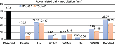
Fig. 10 Comparison of the daily accumulated precipitation on December 9, 2017, at INMET station for MYJ-GF and YSU-KF with all MP schemes.
The best agreement of the MYJ-GF-Goddard configuration to the accumulated daily precipitation is related to the fact that this scheme simulated an anticipated rainfall, which occurs from !4:00 LT, which it is not realistic, since the subtropical storm reached Salvador city at 17:00 LT. Meanwhile, the configuration using YSU-KF was 1-h delayed (Figure 11). Thus, it can be noted that PBL-MYJ, CU-GF and MP-Lin configurations exhibited the most suitable agreement with the observed precipitation data.

3.2 Spatial distribution of wind fields and precipitation
For the WRF model sensitivity analyses, spatial plots of rainfall with wind fields at 10 m were produced to analyze the capture and displacement of subtropical storm Guará over the region. Figure 12 presents the spatial plots of hourly precipitation with wind fields at 10 m between 20:00 and 22:00 UTC (17:00 and 19:00 LT, respectively) at D03 using MYJ-PBL and GF-CU schemes. The choice to show the spatial plots of all runs is to investigate the effect of MP schemes, and also to eliminate the spatial component as the precipitation previous results were compared to a single rain gauge for the entire region. The others were not included as the WRF model presented almost no rain or differences between scenarios.
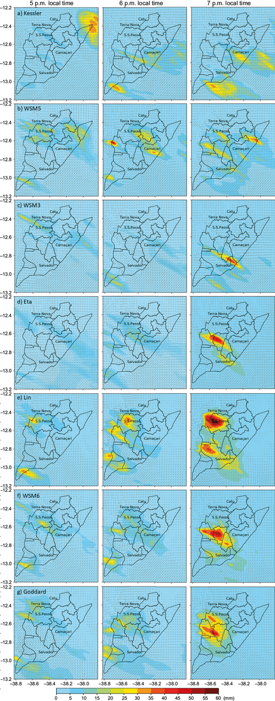
Fig. 12 Spatial distribution of the hourly modeled precipitation with wind fields at 10 m at D03 at 17:00 (left), 18:00 (center) and 19:00 (right) LT for all runs using MYJ-PBL and GF-CU with different MP schemes.
It is simple to distinguish the most suitable MP schemes by visual comparison for this event. The arrival of the subtropical storm was reasonably depicted by Lin, WSM6 and Goddard MP schemes (Fig. 12e-g), which reproduced the evolution of this subtropical storm throughout the hours, with Lin simulation yielding the highest total precipitation rates. Kessler and WSM5 had similar results and emulated the arrival of the event with weak magnitude and patterns precipitation (Fig. 12a, b), despite Kessler is the least complex scheme used. Meanwhile, WSM3 and Eta (Fig. 12c, d) awerend delayed and presented much weaker precipitation fields, therefore they were not suitable for this event. Similar results were found in Sun et al. (2019, who conducted experiments of a typhoon case in South China.
The six-class schemes (Lin, WSM6 and Goddard), which are more complex MP schemes when compared to the other schemes used in the present study, had better performance for this severe event over a Brazilian urban-coastal area. Sikder and Hossain (2016) noted the need to use more complex MP schemes for high rainfall events at high resolution grids since CU schemes are not explicitly employed. Additionally, the inclusion of graupel, which is the hydrometeor class that differs from the others, produced a more realistic precipitation in the region in size and intensity. In Lin and Goddard schemes, graupel is assumed to have a constant bulk density of 400 kg m-3, whereas for WSM6 of 500 kg m-3. However, they also differ in other parameters of the gamma distribution function (Adams-Selin et al., 2013; Han et al., 2013). This analysis revealed that again the most suitable configuration for this weather event was MYJ, GF, and Lin for PBL, CU and MP schemes, respectively, since these schemes appeared to have the most suitable location, shape and intensity of the precipitation.
Figure 13 displays the spatial distribution at 19:00 LT using the MYJ-GF-Lin configuration, and the hourly average contribution of MP and CU schemes to the precipitation of each domain.
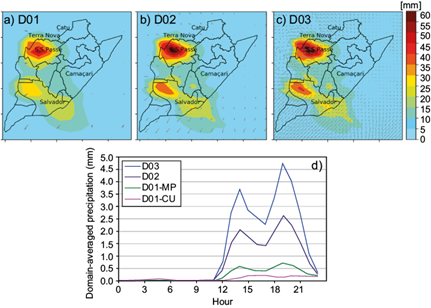
Fig. 13 Average contribution of MP and CU schemes to the precipitation of each domain using PBL-MYJ, CU-GF, and MP-Lin configuration. Spatial plots are depicted at 19:00 LT.
The coarsest domain (D01; Fig. 13a) yielded the lowest rainfall rates, while at a finer resolution (D02 and D03), where the CU scheme was not activated, precipitation was directly produced by the MP schemes. This agrees with Jeworrek et al. (2019), who observed that MP schemes had more impact on precipitation production in mesoscale convective cases. This happens because grid-scale rainfall has to increase its processes to compensate the non-activation of CU parameterization in the finer grids (Sharma and Huang, 2012), thus sub-grid scale motions become better resolved and dominate the total transport and precipitation (Fowler et al., 2016).
As the peak rainfall was registered in the region between 17:00-18:00 LT, rainfall modeled across the entire domain started to be predicted 5 h before the actual peak, with the highest modeled values occurring at 19:00 LT (Fig. 13d). The highest modeled rainfall rates were concentrated over the São Sebastião do Passé (see S.S.Passé in the spatial distribution of Fig.13c) county. Terra Nova and Salvador municipalities, especially over the BTS, also were affected by the subtropical storm Guará. Additionally, over the surrounding areas, where there are large areas of vegetation and water bodies, the wind fields were smaller and divergent. The wind fields agreed with the observed wind roses, which indicates that most of the winds originated from the north, north-northeast, and northeast areas and blew toward the southwest and south-southwest.
The wind rose diagrams (not shown) show that frequency distribution of the observed wind originated from the 25% north, 25% north-northeast, and 33.3% northeast at the INMET station. Meanwhile, the modeled data exhibited a frequency distribution of 20.8, 45.8, and 29.6%. The observed frequency distribution at the Airport station was 33.3% north, 16.7% north-northeast, and 16.7% northeast, while that of the modeled data was 25, 41.7, and 33.3%, respectively. Therefore, the WRF results could depict the same wind sectors with variations in the percentage of frequency distribution and wind magnitudes.
4. Conclusions
Abrupt changes in the atmosphere over coastal-tropical sites are one of the most challenging aspects of atmospheric modeling, particularly for precipitation. Results indicate that the WRF model performed well in the simulation of an extreme rainfall event, i.e., the Guará subtropical storm. Although several studies have already been conducted on this subject in other regions, the best model configuration will depend on the area under analysis. This constitutes the first study evaluating physical parameterization schemes over the MRS in Brazil, using the WRF model.
Several configurations combining different PBL, CU, and MP schemes were tested in our study. Although the results are based on a single case study, significant differences could be seen on the hourly variation of meteorological parameters. The PBL-MYJ, CU-GF, and MP-Lin schemes were selected to generate the spatial and temporal distribution plots, and the wind roses, as this combination agreed with the main variable best. The precipitation production was majorly influenced by the microphysics scheme when compared to the cumulus scheme in D01. The model represented well the arrival and occurrence of this extreme weather event in a tropical and coastal region, considering that the region already had intense convective characteristics and was constantly influenced by sea breezes, which could interfere in the model results and compromise the performance of the simulations. The WRF model could represent phenomena that occur in the PBL reasonably well, justifying its application at an urban scale. Over the past 15 years, the MRS region has experienced industrialization and urbanization, which may have caused the weather station to become poorly located. Furthermore, one rain gauge was available for the entire region to compare with the WRF data, indicating that the model validation could be better conducted with more observational data, which is a limitation of the study. The results demonstrate that schemes must be thoroughly validated using additional experimental observations, such as Light Detection and Ranging and Sonic Detection and Ranging measurements. In addition, future work should include the analyses of more cases, and also other environmental conditions to reach definitive conclusions in the use of the selected schemes.

