


 text new page (beta)
 English (pdf)
 Article in xml format
 Article references
 Send this article by e-mail
 Cited by SciELO
  Similars in
SciELO
Similars in
SciELO 
 Permalink
1. Introduction
Article 2 of the Paris Agreement (United Nations, 2015) suggests “holding the increase in the global average temperature (∆T) to 2 ºC and pursuing efforts to limit the temperature increase to 1.5 ºC above pre-industrial levels.” Hence, this paper analyses likely human bioclimatic conditions in Mexico for climate change scenarios with time horizons in which global average temperature (∆T) reaches 1.5 ºC and 2 ºC. The 1 ºC time horizon has been added as an extra tool for decision makers to consider when discussing regulations on residential electricity consumption for air conditioning on the 30 metropolitan areas that had more than half a million inhabitants in 2010 (Table I).
Table I Metropolitan areas (abbreviations in parentheses) with populations of at least half a million in 2010 (INEGI, 2010) and in 2030 (CONAPO, 2006).
| Metropolitan area | Population (thousands) 2010/2030 | Metropolitan area | Population (thousands) 2010/2030 |
| Valley of Mexico (VMx) | 20 117/23 247 | Acapulco (Acap)* | 863/959 |
| Guadalajara (Gdl) | 4 435/5 515 | Tampico (Tamp)* | 859/1 036 |
| Monterrey (Mty)* | 4 106/5 362 | Chihuahua (Chih) | 852/1 058 |
| Puebla-Tlaxcala (Pue-Tlax) | 2 729/3 315 | Morelia (Mor) | 830/958 |
| Toluca (Tol) | 1 936/2 652 | Saltillo (Salt) | 823/1 052 |
| Tijuana (Tij) | 1 751/2 335 | Veracruz (Ver)* | 812/926 |
| León (León) | 1 610/1 888 | Villahermosa (Vhsa)* | 755/926 |
| Juárez (Jrez) | 1 332/1 616 | Reynosa-Río Bravo (Reyn)* | 727/960 |
| La Laguna (Lag)* | 1 216/1 502 | Tuxtla Gutiérrez (TuxG)* | 684/873 |
| Querétaro (Qro) | 1 097/1 450 | Cancún (Ccún)* | 677/1 129 |
| San Luis Potosí (SLP) | 1 040/1 259 | Xalapa (Xal) | 666/788 |
| Mérida (Mér)* | 973/1 246 | Oaxaca (Oax) | 608/703 |
| Mexicali (Mxli)* | 937/1 210 | Celaya (Clya) | 602/699 |
| Aguascalientes (Ags) | 932/1 188 | Poza Rica (Prica)* | 514/581 |
| Cuernavaca (Cuer)* | 925/1 150 | Pachuca (Pach) | 512/664 |
* Indicates warm or hot areas.
Since the goal of this paper is to estimate the human bioclimate conditions and their effects on residential electricity consumption in Mexico for the rest of the century, warming due to urbanization was added to the global climate change scenarios.
Increase of heat in cities because of urbanization, i.e., urban heat island (UHI), adds up to thermal gain due to climate change. The air in the urban canopy of UHIs is usually warmer than that of the surrounding countryside (Oke, 1987). The combination of these effects will lead to an increase in demand of electricity for air conditioning (AC) to cool indoor areas. Cities that so far can manage without AC will have to add them gradually. The results of Wan et al. (2011) for different climates, especially for Australia (Wang et al., 2010), California (Xu et al., 2012), and Canada (Berardi and Jafarpur, 2020) show that heating will decrease in cities with cold or temperate climates during the summer and, most likely, in all cities during winter.
Previous research in Mexico has estimated changes in human bioclimatic conditions under climate change scenarios. Jáuregui and Tejeda-Martínez (2001) estimated human comfort conditions in Mexico City for a possible doubling of atmospheric CO2 but the UHI effect was not considered. Tejeda-Martínez and Rivas (2003) analysed similarly south-eastern Mexico while Rodríguez et al. (2004) and García and Tejeda-Martínez (2008) analysed the state of Veracruz. García et al. (2010) studied three cities in north-western Mexico. Luyando and Tejeda-Martínez (2010) dealt with the expected bioclimate halfway through the 21st century in five urban regions in Central Mexico, located 2200m above sea level. Luyando (2016) assessed bioclimatic adjustments in Mexico City for the second half of the 21st century as a result of global climate change and urban heating.
Figure IV.2.2 (p. 167) of the 4 th National Mexican Memorandum about Climate Change (SEMARNAT-INE, 2010) is a summary of Tejeda-Martínez et al. (2011), which measured the average thermal stress conditions in ten urban areas with more than one million inhabitants in the last decade of the 20th century. It shows estimates of electricity consumption by user in the first decade of the 21st century; projections for 27 cities are presented for time horizons in 2020, 2050, and 2080.
This paper uses the notion of thermal comfort as described by the American Society of Heating, Refrigerating and Air-Conditioning Engineers, which defines it as “[joint] condition[s] of mind which expresses satisfaction with the thermal environment” (Berglund et al., 1997). A common, indirect way to assess thermal sensation is through bioclimatic comfort indices.
Epstein and Moran (2006) and Blazejczyk et al. (2012) concur in classifying the indices into three groups: 1) rational indices, based on the general equation of thermal balance; 2) empirical indices, based on objective and subjective strain; and 3) direct indices, based on direct measurements of environmental variables. The first two groups depend on many variables, some of which require uncommon specific measurements such as radiant temperature of the environment, globe temperature, inner walls’ temperatures, and occupants’ skin temperatures. The third group is easier to use and apply because it depends on environmental variables. Although these direct indices are relatively old, they are still in use in human bioclimate studies, and perform satisfactorily when compared to sophisticated indices.
Many human bioclimate studies coincide that room temperature, atmospheric humidity, solar radiation, radiation emitted by the surroundings, and wind are the main environmental elements in human thermal sensation (Auliciems and De Dear, 1998). Only indices that depend solely on the temperature and relative humidity are useful enough, since wind and solar radiation can be controlled indoors.
More than 160 indices have been used to assess human bioclimate in the last 100 years (De Freitas and Grigorieva, 2015). The most sophisticated ones simulate the physical and physiological conditions present in the feeling of human comfort. In contrast, the simplest ones use only room temperature and atmospheric humidity as input data. Apparent Temperature, Effective Temperature, and the Humidex are among those that depend on these last two variables (Anderson et al., 2013; Chirico and Magnavita, 2019; Binarti et al., 2020).
Blazejczyk et al. (2012) found a high coefficient of determination (97%) between Effective Temperature - a direct index- and the Universal Thermal Comfort Index (UTCI) - a sophisticated index that focuses on physiological adaptation -. According to Auliciems and De Dear (1998), the PMV index and Effective Temperature are the best options to quantify the physiological human response to the thermal environment.
De Freitas and Grigorieva (2017) recently classified and evaluated 165 bioclimatic indices using six evaluation criteria: validity, usability, transparency, sophistication, completeness, and scope under different environmental conditions, assigning up to a maximum score of 30. Effective Temperature stands out with a score of 23, followed by Humidex with 15. Although the Humidex has an average rating, it is found in a number of recent publications on climate change (Oleson et al., 2015; Orosa et al., 2014a; Orosa et al., 2014b; Kum and Celik, 2014; Giannakopoulos et al., 2011), heat waves (Stewart et al., 2017; Lee et al., 2016; Hamdi et al., 2016; Kravchenko et al., 2013; Kershaw and Millward, 2012; Mastrangelo et al., 2007), urban environments (Roshan et al., 2017; Charalampopoulos et al., 2013), and the energy sector (Yildiz et al., 2017; Miller et al., 2017; Marvuglia and Messineo, 2012; Beccalli et al., 2008).
Jáuregui et al. (1997) and Moran and Epstein (2006) showed that if some variables in a complex index are parameterized, its sensitivity and variability are reduced to those of a simple index. Therefore, bioclimatic evaluations based on temperature and humidity variables are still valid.
Hence, this research will use the Effective Temperature index and the Humidex. Preliminary results to those shown in this article appeared in INECC-PNUD (2017a) and SEMARNAT-INECC (2018).
2. Data and Methods
2.1 Data
Mexico, due to its geographic location, experiences mid-latitude meteorological systems in winter and tropical systems in summer. It is also affected by topography and ocean-continent convergence (Mosiño and García, 1974). Thus, we find a great variety of climates that range from hot, with average annual temperatures above 32 ºC, to cold, with temperatures below 10 ºC, but average annual temperatures in almost 90% of the country range from 10 ºC to 26 ºC. As a whole Mexico has 23% hot-subhumid, 28% dry, 21% very dry, and 21% temperate-subhumid climates (Magaña, 1999).
The dataset used is known as CLICOM (National Climatological Database), based on the Mexican climatological station network, for the period 1980-2009. The website managed by the Mexican research center CICESE (http://clicom-mex.cicese.mx) provides daily maximum and minimum temperature data. Inconsistent records were discarded, for example, those where the daily maximum temperature was lower than the minimum one and vice versa. Stations with less than 80% of the data were not taken into account. Because of this, calculations for Chihuahua, Reynosa-Río Bravo, and Pachuca used the reanalysis database of Livneh et al. (2015). The spacing of its 1/16 mesh has currently one of the highest resolutions, which provided acceptable values at the required points. The database is also valid for stations with time frames longer than 20 years.
The National Institute of Ecology and Climate Change, and the United Nations Development Programme (INECC-PNUD, 2017b) provided the climate change projections. Output of the GFDL-CM3 and HADGEM2-ES models were used, with radiative forcings RCP4.5 and RCP8.5 for three time horizons that reach increases in the global average temperature of 1.0 ºC (years 2030 to 2048), 1.5 ºC (2041-2066), and 2.0 ºC (2051-2100).
The National Population Council (CONAPO, 2006) provided data on family size in 2010, population projections for 2030, average family size projections for 2010-2030, population projections for 2030 by district and town to determine future scenarios of population growth, and electricity consumption by user for cooling needs in 2010 with projections for 2030.
2.2 Selected bioclimatic index(es)
The Humidex was developed in Canada in 1965 and modified by Masterton and Richardson (1979). Its algebraic expression is:
where Ta is the room temperature in ºC and e is the water vapour pressure in hPa.
Effective Temperature (ET) can be expressed as (Missenard, 1933):
Here, the relative humidity (f) is given in decimals.
Only the Humidex was used here since results between using Effective Temperature or Humidex did not vary significantly when converting indices into cooling needs (as energy units, kW-user per year, for example).
2.3 Hourly hygrothermal data
Temperature and relative humidity hourly data are required to compare the bioclimatic conditions of 2010 to future ones. Since some files of National Climatological Database (CLICOM database) do not have humidity data, these were obtained by averaging mean monthly extreme temperatures. Comparing base and future scenarios is possible if the same calculation method is used in both.
The average monthly relative humidity was calculated as the ratio of the average monthly vapour pressure e (in hPa) and the average monthly saturation vapour pressure e s (in hPa). Atmospheric humidity data are rare in climatological station networks. Hence, e was calculated by the polynomial proposed by Tejeda-Martínez and Rivas (2003), which is dependent of the average monthly minimum temperature T m :
e s was obtained from Adem (1967), using the mean monthly temperature T:
The average monthly minimum relative humidity (f min ) was obtained by combining the monthly mean e with the e s as a function of the mean maximum temperature (e stmax ). The average monthly maximum relative humidity (f max ) is derived from the monthly mean e s as a function of the mean minimum temperature (e stmin ):
f min = e/ e stmax and f max = e/ e stmin
Monthly averages of hourly data were obtained from the equations proposed and used by Tejeda-Martínez (1991), and Tejeda-Martínez and Rivas (2003):
where T hor and f hor are the hourly temperature and relative humidity (in ºC and decimals, respectively); a, b, and c for latitudes south of the Tropic of Cancer have values of 0.096, 2.422 and -0.339, respectively. For the tropics and latitudes to the north, values are 0.026, 3.190 and -0.375 (from March to October) and 0.023, 3.436 and -0.421 (from November to February); t is the time of day from sunrise; T max , T min , f max and f min are the average monthly maximum and minimum relative temperatures and humidity for the period 1980-2009 at the selected cities in this study.
Monthly averages or hourly data on temperature, relative humidity, and vapor pressure - which remained unchanged throughout the daytime - were obtained using this method to generate monthly Humidex values (Equation 1).
2.4 Base and future bioclimatic conditions
For the base period (1980-2009) and climate change scenarios, thermal comfort conditions (monthly, seasonal, and annual) of thirty metropolitan areas (Table I) were analysed. Equations 5 and 6 were substituted in the equations of the selected bioclimatic indices to generate the hygrothermal sensation base period 1980-2009. This sensation is defined as a response to the state of thermoreceptors in a human body and describes how the person feels hygrothermically (Parsons, 2014). It is commonly categorized into cold, cool, slightly cool, neutral, slightly warm, warm, and hot (ASHRAE, 2004). This calculation requires to know the neutral temperature -also called comfort or preferential temperature, or thermopreferendum, T p ). For Auliciems (1983), T p shows the thermal preference of the inhabitants acclimatized to a particular site. The International Union of Physiological Science defined it as “conditions which an individual, organism or a species selects for its ambient environment” (Bligh and Johnson, 1973). There are different models to estimate this value, such as those by García and Tejeda-Martínez (2008), and Martínez et al. (2017). The most-often used equation for tropical latitudes was applied (T is the average monthly temperature in ºC):
The preferred monthly values for each comfort index were calculated from T p and f = 0.5. The comfort interval was established as T p ± 1.5 ºC.
INECC-PNUD (2017b) provided the temperature increases due to climate change; these were added to the average monthly hourly values of the base period 1980-2009. This is how we obtained the preferred bioclimatic scenario with climate change. The warming effect due to urbanization, UHI, was also added. According to Jáuregui (1986), the UHI’s maximum intensity (HI max ) in tropical cities, in ºC, is obtained from population in the urban area (P) as:
It is acknowledged that the UHI does not occur in the entire urban area (Tejeda-Martínez et al., 2011); it decreases from the centre towards the periphery and has a daily and an annual variation. Using INEGI’s (National Institute of Statistics and Geography) information, Luyando (2016) estimated the UHI’s intensity for each basic geographic area. The result, applied here, was one sixth of the maximum intensity calculated with Equation 8. Equation 9 was used in this analysis to estimate the UHI’s temperature increase for each of the weather stations at the metropolitan areas studied and each scenario:
The population forecast (P) as the number of inhabitants in each urban area for the 2030s was used for future projections (Table I, approximately when the 1 ºC mean global warming time horizon is met). The value remained unchanged since CONAPO (2006) calculates that the national population will undergo a very slow growth from 2030.
2.5 Electricity consumption
Heat degree hours (HDH), corresponding to heating needs, and cold degree hours (CDH), for cooling needs, were calculated as:
hum i are the Humidex’s average monthly hourly values, R min is the lower limit (calculated with f = 0.5 and T p -1.5 ºC), and R max is the upper limit (calculated with f = 0.5 and T p + 1.5 ºC) of the Humidex comfort interval. This useful and simple method is well-known, applied to Istanbul by Durmayaz et al. (2000) and by Assawamartbunlue (2013) in Thailand.
De Buen (2017) estimated annual electricity consumption for comfort in each residential electricity rate (1, 1A, 1B, 1C, 1D, 1E or 1F). These rates are established from the highest average monthly temperatures in three consecutive months over a period of five years, as stated in the Federal Official Gazette (DOF, 2002). Results by De Buen (2017) were used to convert values to energy needs (in kWh, per electric service user). The 30 metropolitan areas were classified according to their electricity rate; an average CDH was taken from those with the same rate. The last column of Table II shows these equivalencies. Since the rate districts 1 and 1A had no data on average annual consumption for comfort, they got the same values of rate 1B.
Table II Residential electricity rates (DOF, 2002), metropolitan areas and equivalences of CDH to kWh-user.
| Electricity rates | Metropolitan areas (alphabetical order) | Equivalences of CDH to kWh-user |
| 1 | Aguascalientes, Celaya, Cuernavaca, Guadalajara, León, Morelia, Oaxaca, Pachuca, Puebla-Tlaxcala, Querétaro, Saltillo, San Luis Potosí, Tijuana, Toluca, Xalapa and Valley of Mexico. | 0.0055 |
| 1 B | Acapulco, Chihuahua, Poza Rica y Tuxtla Gutiérrez. | 0.0055 |
| 1 C | Cancún, Juárez, La Laguna, Mérida, Monterrey, Tampico and Veracruz | 0.0153 |
| 1 D | Villahermosa | 0.0145 |
| 1 E | Reynosa-Río Bravo | 0.0477 |
| 1 F | Mexicali | 0.0829 |
We established, as a working hypothesis, that consumption will increase not only because of the CDH’s growth due to global and local climate change, but also because of economic factors. AC systems, fans, and refrigerators are increasingly cheaper. De Buen (2017) documented this increase in consumption from 2012 to 2016. The technology in these devices tends to be more efficient and more AC solutions are passively introduced in housing. It is expected that the increase in AC use due to accessibility will cancel out the decrease due to better technology. Hence, the CDH equivalence for electricity consumption in the base period will remain the same in the future. Note that the CDH calculations include the acclimatization of the subjects to the thermopreferendum or preferred temperature.
The term “user” in De Buen (2017) refers to electricity meter or the household with an electric service meter. Therefore, to obtain the consumption for cooling per inhabitant, the value gets divided by the average number of people in a household as INEGI registered it for the base period in 2010 (3.19 people per family), and CONAPO’s projections for the scenarios ΔT = 1.0 ºC (year 2030; 3.17 people per family), ΔT = 1.5 ºC, and 2.0 ºC (year 2050; 3.01 people per family).
The total consumption of each metropolitan area was evaluated for the base period and for 2030 and 2050 (for example, see Table III). On the other hand, as an energy equivalence regarding the decrease in heating needs (HDH) was not found in the literature, just the reduction percentage was reported (Table IV).
Table III Increased electrical consumption (%) for ΔT=2.0 ºC with respect to the base period (climatology 1979-2012 and population 2010), for warm and hot metropolitan areas.
| Metropolitan area | Increased electrical consumptions (%) | ||||||
| Without UHI | With UHI | ||||||
| Yearly | Winter | Summer | Yearly | Winter | Summer | ||
| Monterrey | 212 | 336 | 185 | 247 | 417 | 210 | |
| La Laguna | 107 | 85 | 112 | 132 | 122 | 134 | |
| Mérida | 163 | 172 | 156 | 196 | 210 | 186 | |
| Mexicali | 130 | 210 | 107 | 139 | 234 | 112 | |
| Cuernavaca | 447 | >1000 | 346 | 573 | >1000 | 432 | |
| Acapulco | 84 | 90 | 79 | 90 | 98 | 83 | |
| Tampico | 140 | 218 | 115 | 159 | 264 | 126 | |
| Veracruz | 117 | 139 | 103 | 132 | 161 | 114 | |
| Villahermosa | 130 | 176 | 107 | 144 | 204 | 114 | |
| Reynosa-Río Bravo | 184 | 254 | 165 | 206 | 298 | 181 | |
| Tuxtla Gutiérrez | 192 | 221 | 176 | 219 | 259 | 197 | |
| Cancún | 205 | 235 | 186 | 226 | 266 | 200 | |
| Poza Rica | 136 | 192 | 116 | 155 | 228 | 130 | |
Table IV Decrease in heating needs (%) for ΔT=2.0 º with respect to the base period (climatology 1979-2012 and population 2010).
| Metropolitan area | Without UHI | With UHI | ||||
| Annual | Winter | Summer | Annual | Winter | Summer | |
| Valley of Mexico | 38 | 34 | 44 | 52 | 46 | 61 |
| Guadalajara | 52 | 45 | 66 | 63 | 57 | 76 |
| Monterrey | 47 | 45 | 60 | 59 | 57 | 75 |
| Puebla-Tlaxcala | 31 | 27 | 37 | 40 | 35 | 48 |
| Toluca | 20 | 18 | 23 | 26 | 23 | 30 |
| Tijuana | 37 | 38 | 37 | 46 | 46 | 47 |
| León | 40 | 34 | 51 | 49 | 42 | 63 |
| Juárez | 28 | 25 | 36 | 33 | 30 | 43 |
| La Laguna | 27 | 24 | 43 | 36 | 32 | 54 |
| Querétaro | 35 | 31 | 42 | 44 | 39 | 53 |
| San Luis Potosí | 29 | 26 | 33 | 36 | 32 | 41 |
| Mérida | 67 | 63 | 75 | 79 | 76 | 86 |
| Mexicali | 37 | 35 | 42 | 44 | 41 | 52 |
| Aguascalientes | 35 | 29 | 47 | 43 | 36 | 57 |
| Cuernavaca | 61 | 54 | 76 | 72 | 65 | 88 |
| Acapulco | 0 | 0 | 0 | 0 | 0 | 0 |
| Tampico | 87 | 87 | 100 | 97 | 96 | 100 |
| Chihuahua | 28 | 24 | 38 | 33 | 28 | 44 |
| Morelia | 31 | 28 | 36 | 38 | 34 | 44 |
| Saltillo | 38 | 30 | 64 | 44 | 35 | 74 |
| Veracruz | 100 | 100 | 0 | 100 | 100 | 0 |
| Villahermosa | 0 | 0 | 0 | 0 | 0 | 0 |
| Reynosa-Río Bravo | 49 | 47 | 64 | 57 | 55 | 75 |
| Tuxtla Gutiérrez | 79 | 76 | 99 | 88 | 87 | 100 |
| Cancún | 0 | 0 | 0 | 0 | 0 | 0 |
| Xalapa | 38 | 34 | 44 | 46 | 42 | 54 |
| Oaxaca | 43 | 36 | 54 | 51 | 44 | 65 |
| Celaya | 33 | 32 | 35 | 41 | 38 | 45 |
| Poza Rica | 76 | 75 | 100 | 87 | 86 | 100 |
| Pachuca | 27 | 25 | 29 | 33 | 30 | 36 |
3. Results
Estimated AC needs were calculated from the Humidex, with results from the GFDL-CM3 and HADGEM2-ES models and two radiative forcings (4.5 and 8.5 Wm-2). The results shown here correspond to the combination of the Humidex with HADGEM2-ES and a forcing of 8.5 Wm-2. This combination was chosen because HADGEM2-ES showed greater sensitivity and the forcing of 8.5 Wm-2 for future cooling needs has precautionary value.
The thermal increases by UHI (from Equation 9) range from 1.1 ºC, for the metropolitan area of the Valley of Mexico, to 0.6 ºC for Poza Rica. Thus, they are lower than the climate change horizons (1.0 ºC, 1.5 ºC and 2.0 ºC).
Figure 1 shows the annual cooling needs in CDH for all 30 urban centers for the base period, while Figure 2 shows the annual increases in consumption for cooling per inhabitant at horizons ΔT = 1.0 ºC, 1.5 ºC and 2.0 ºC, with and without the UHI. The largest hygrothermal rise is expected in coastal metropolitan areas or near the eastern and southern coasts (Fig. 1). Increases in consumption for cooling are expected to be higher in the metropolitan areas of Mexicali, Reynosa-Río Bravo, Cancún, Villahermosa, Veracruz, Tampico, Monterrey, Mérida, and Ciudad Juárez when converting to energy units per inhabitant (Fig. 2). Note that Ciudad Juárez is located at 1120m above sea level, while all others are below 1000m above sea level. These are followed by Tuxtla Gutiérrez, Acapulco, and Poza Rica, also located below 1000m above sea level.
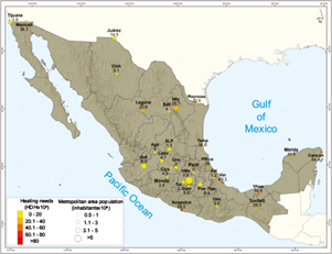
Fig. 1 Annual cooling needs (cold degree hours, CDH) for base period (climatology 1979-2012 and population 2010).
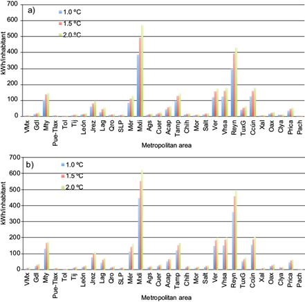
Fig. 2 Annual increases in consumption for cooling (kWh/inhabitant) for time horizons that will reach increases in the average global temperature (∆T) of 1 ºC, 1.5 ºC and 2 ºC. a) without UHI, b) with UHI.
Increases will grow in time, from one ΔT horizon to another, and it is expected to be even larger in the presence of UHIs. These increases will be higher from March to August (summer) and will decrease slightly from September to February (winter).
Figure 3, similar to Figure 2 but applied to the entire population in each metropolitan area, shows increases in cooling needs. Monterrey has a larger expansion because of its population. While usage in metropolitan areas in central Mexico will increase minimally, none of them display a reduction in consumption for cooling.
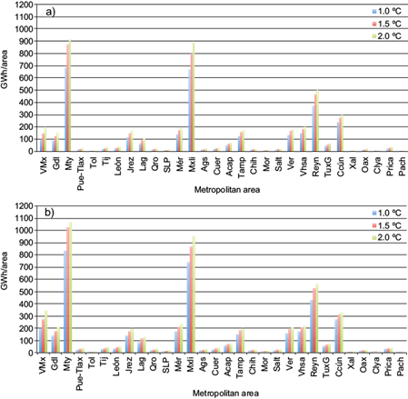
Fig. 3 Annual increases in consumption for cooling (GWh/area) for time horizons that will reach increases in the average global temperature (∆T) of 1 ºC, 1.5 ºC and 2 ºC. a) without UHI, b) with UHI.
Table III presents the percentage increase in consumption needs for cooling compared to the base period (averages from 1979 to 2012, population from 2010) in warm or semi-warm metropolitan areas for the climate change scenario ∆T = 2.0 ºC. It is clear that population growth contributes the most to increases in energy consumption.
Figure 4 shows the base period of annual heating needs in Heat Degree Hours (HDH). These values were used to calculate the percentage reductions in Figure 5. As noted above, it was not possible to find energy equivalences because of a lack of conversion from HDH to energy units in the literature.
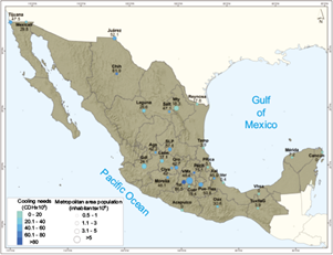
Fig. 4 Annual needs of heating (hot degree hours, HDH) for base period (climatology 1979-2012 and population 2010).
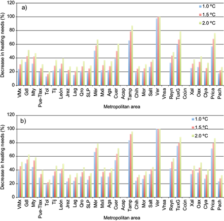
Fig. 5 Decrease in heating needs (%) for time horizons that will reach increases in the average global temperature (∆T) of 1 ºC, 1.5 ºC and 2 ºC. a) without UHI, b) with UHI.
Acapulco, Villahermosa, and Cancún did not use heating during the base period and, thus, show no reduction in future heating use; similarly for Veracruz during the summer months (March-August). The decline in heating needs increases as time horizons progress (ΔT = 1.0 ºC, 1.5 ºC and 2.0 ºC).
It is predicted that the largest decrease in heating needs will occur during summer when considering UHI in all metropolitan areas considered. The metropolitan areas of Tampico and Poza Rica show a 100% decrease in heating needs from time horizon ΔT = 1.0 ºC for summers with UHI; Tuxtla Gutiérrez will reach the same decline from horizon ΔT = 1.5 ºC. This means that the small heating demands during the early morning hours -usually solved by the building’s thermal inertia or clothing- will disappear completely in summer. Similar results are found for the metropolitan areas of Valley of Mexico, Guadalajara, Monterrey, León, Mérida, Cuernavaca, Saltillo, Reynosa, and Oaxaca. These areas are expected to have a significant gradual decrease close to or over 60% in heating use for time horizon ΔT = 2.0 ºC when the UHI is considered. This reduction means less need for shelter and heating use in cool mornings.
All analysed metropolitan areas show a decrease of at least 15% for heating needs for winter (results not shown) without considering the UHI; decreases will be less when considering the UHI.
The metropolitan areas that combine both an increase in cooling needs and a decrease in heating needs are Reynosa, Monterrey, Tampico, Mérida, Veracruz, Poza Rica, and Tuxtla Gutiérrez, mainly during summer and considering the UHI. All the analysed metropolitan areas will experience increases in both minimum and maximum temperatures, leading to higher cooling needs and a decrease in heating use.
Table IV shows the decrease in heating needs for ΔT = 2.0 ºC compared to the base period. Metropolitan areas that in the base period did not have heating needs, show a 0% decrease. Those with a decrease of 100% or close to 100% can gradually abstain from heating.
4. Discussion
The methods and results of this study -decreasing heating needs and increasing cooling needs due to climate change- are consistent with those published by Petri and Caldeira (2015) for 25 cities in the United States, Mourshed (2011) for Dhaka and Bangladesh, Christenson et al. (2006) for four cities in Switzerland, and Schoetter et al. (2020) for Toulouse and Dijon in France.
Table V shows the increase intervals in electricity consumption for cooling per inhabitant. This is expected to exceed the 100 kWh per inhabitant in metropolitan areas, and ranges from a minimum increase (ΔT = 1 ºC without UHI) to a maximum one (ΔT = 2 ºC with UHI). The largest increase will occur in northern Mexico and in urban coastal areas of the Gulf of Mexico and the Caribbean. As previously mentioned, the results of the works cited in the introduction and those of this work correspond in order of magnitude to the percentage of consumption per inhabitant.
Table V Metropolitan areas that will increase their cooling needs per inhabitant by more than 100 kWh (see Figure 2).
| Metropolitan area | ΔT = 1 ºC without UHI (kWh/inhabitant) | ΔT = 2 ºC with UHI (kWh/inhabitant) |
| Mexicali | 390 | 610 |
| Reynosa | 300 | 500 |
| Villahermosa | 110 | 200 |
| Cancún | 120 | 200 |
| Veracruz | 110 | 200 |
| Monterrey | 100 | 180 |
| Tampico | 100 | 170 |
| Mérida | 90 | 150 |
| Juárez | 60 | 105 |
Time trends in decadal consumption for four representative areas are shown in Figure 6. As an example, Puebla-Tlaxcala displays a similar behaviour to other temperate zones, such as Toluca, León, Morelia, San Luis Potosí, Aguascalientes, Querétaro, Tijuana, and even the Valley of Mexico. The main difference is the population size in each of them. The trend seen for Monterrey is representative of the pattern seen in other northern warm areas during summer such as Mexicali, Ciudad Juárez, La Laguna, Saltillo, and Reynosa. Note that cooling needs in these northern areas are almost independent of the UHI. This is slightly different in metropolitan areas of the humid tropics like Cancún, Veracruz, Tampico, Acapulco, Tuxtla Gutiérrez, Mérida, and Villahermosa. Three areas are an exception: Celaya, Poza Rica, and Pachuca. CONAPO estimates that population in those areas will decline before mid-century.
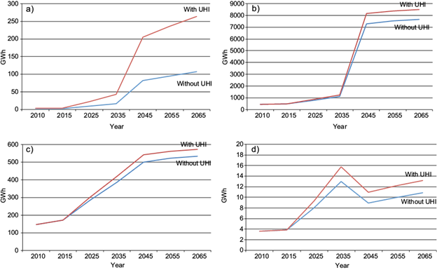
Fig. 6 Four examples of decadal consumption trends: a) Puebla-Tlaxcala, b) Monterrey, c) Cancún, d) Celaya.
Heating needs are certainly expected to decrease under global and local warming scenarios due to urbanization. Results of this study show that the percentage reduction (over 50%) will be greater in warm places like Mérida, Tampico, Veracruz, Tuxtla Gutiérrez, and Poza Rica. Acapulco and Cancún already used no heating in the base period. Cold areas like Toluca, Pachuca, and Tijuana will decrease use by 15 to 30%, considering the UHI. The decrease in the remaining areas will be between 25 and 60%. However, it is important to note that temperate metropolitan areas (Aguascalientes, Celaya, Cuernavaca, Guadalajara, León, Morelia, Oaxaca, Pachuca, Puebla-Tlaxcala, Querétaro, Saltillo, San Luis Potosí, Tijuana, Toluca, Xalapa, and Valley of Mexico) experience extreme minimum temperatures below 5 ºC in the base period, and it is very likely that cold waves will continue to affect them in the future.
5. Recommendations
Some regions of the country have already experienced a shortage of electricity due to excessive demand derived from AC use (Loret de Mola, 2017; Arias, 2019; ADN, 2019). This study shows that the situation will worsen in the future. Moreover, cold urban areas, like Toluca, Pachuca, and Tijuana, have also experienced heat waves increasing AC demand. Recommendations resulting from this analysis point towards a need to reduce AC energy consumption through measures inside buildings and in urban environments, as well as to develop awareness campaigns.
There is a sustainable building framework in Mexico for residential areas (CONAVI, 2010) but it is not mandatory. There are also two official Mexican standards issued with the purpose of reducing energy consumption from AC in buildings: NOM-018-ENER-2011 (Thermal Insulation for Buildings. Features and Test Methods), and NOM-020-ENER- 2011 (Energy Efficiency in Construction. Building Enclosures for Residential Use). Although both are mandatory, their compliance is not truly monitored. There are also some voluntary Mexican technical standards: NMX-AA-164-SCF1-2013 (Sustainable Building: Minimum Environmental Criteria and Requirements), NMX-AA-171-SCFI-2014 (Requirements and Specifications of Environmental Performance in Lodging Facilities), and NMX-AA-SCFI-157-2012 (Sustainability Requirements and Specifications for Site Selection, Design, Construction, Operation, and Abandonment of Tourist Property Development Sites in Coastal Areas of the Yucatán Peninsula).
Local government needs to embrace these regulations and, together with state and federal governments, promote, monitor, and implement those regulations. It is also recommended that energy providers (particularly, the Federal Electricity Commission, CFE) get involved in monitoring compliancy with NOM-018 and NOM-020 official standards, ensuring that all new and renovated properties comply with these regulations.
Important measures have been implemented in the last decade. For example, the National Workers Housing Fund (INFONAVIT) started the Green Mortgage Program, which grants an additional credit for eco-technologies that save water, electricity, and gas. These technologies include solar heaters, thermal insulation, energy saving lighting, etc. The National Housing Council launched “This is Your Home”, a program that links subsidies to a series of criteria that guarantee property’s sustainability.
The government of Mexico City (formerly the Federal District) issued a Sustainable Building Certification Program in 2008. It established a standard to reward residential and commercial buildings with tax or financial incentives. However, most of these buildings have been built by large commercial developers and have been certified by international standards, namely LEED (Leadership in Energy and Environmental Design) rather than by individuals. LEED and similar labels, do not correspond with Mexico’s socioeconomic, cultural, and technological aspects and cannot be applied nationwide.
It is recommended that each metropolitan area incorporates new regulatory codes to current urban development regulations. Construction licenses should include compliance with energy efficiency and sustainable building measures. For example, a building’s thermal load or an energy simulation could be listed as prerequisite to obtain licenses for building construction or remodelling. This is similar to the Building Energy Certificate required for developers in the European Union. It is, therefore, paramount that municipal authorities, research centers, professional associations, and industrial chambers of construction and housing work together towards achieving the same goal.
UHI intensity tend to increase morbidity and mortality in children and the elderly. In Mexico City, for example, children between the ages of 0 and 14 suffer acute diarrhoea as a consequence of the UHI and climate change (Vargas and Magaña, 2020). In Barcelona, Spain, from 1992 to 2015, elderly men and women were the most vulnerable groups (Ignole, et al, 2020).
Mitigation of UHIs requires a higher density of green areas. The aforementioned standard NMX-AA-164-SCF1-2013 (for Sustainable Building) establishes that the percentage of free areas must be 10% larger than the minimum value established by local regulation, without parking areas. Moreover, these common areas for users and visitors should allow water infiltration.
Ventilation should also be promoted. Rows of tall buildings on the seashore often disturb the local sea breeze regimes in coastal cities. New real estate developments should therefore consider fresh wind corridors to enhance ventilation of residential areas. However, in humid climates, adding more humidity to the environment can increase the intensity or duration of hygrothermal discomfort, which could lead to increased installation of AC systems. Particularly in urban environments where promoting ventilation may be difficult, mitigating the UHI’s intensity would not only lead to energy savings, but would also ease the strength of heat waves and promote better quality of life.

