


 text new page (beta)
 English (pdf)
 Article in xml format
 Article references
 Send this article by e-mail
 Cited by SciELO
  Similars in
SciELO
Similars in
SciELO 
 Permalink
1. Introduction
An interest in determining the natural and anthropogenic trends of carbon dioxide (CO2) began in the 1950s after C.D. Keeling performed the first continuous measurements to establish a global atmospheric record (Keeling, 1960). The amount of CO2 in the atmosphere is regulated by a balanced exchange with the Earth’s oceans, biosphere, and geosphere. However, recent human activities related mostly to fossil fuel combustion and land-use changes have resulted in a 47% increase in the global average CO2 concentration, from 277 ppm at the beginning of the pre-industrial era (i.e. 1750) to 407 ppm in 2018 (Friedlingstein et al., 2019).
It has been estimated that people living in urban areas use up 78% of the world’s consumed energy and are responsible for emitting more than 60% of the anthropogenic CO2, which implies that mitigation strategies adopted by city and local governments could be the most effective to slow the current growth in ambient Greenhouse Gas (GHG) concentrations (World Bank, 2010; Bazaz et al., 2018). Efficient mitigation policies hinge on having realistic estimates of the intensity and distribution of sinks and sources of CO2 in the landscape. However, emissions from urban environments are commonly estimated from inventories of fixed and mobile sources, emission factors and usage data, a type of bottom-up methodology associated with considerable uncertainty (Marland et al., 2009) and updated infrequently. Recent studies have shown that in addition to thorough inventories, a combination of continuous monitoring of CO2 dry mole fraction at surface stations and atmospheric transport modelling are required for a verifiable quantification of the emissions landscape in a complex urban environment (Lauvaux et al. 2013; Bréon et al., 2015; Turnbull et al., 2014; Leip et al., 2017; Wu et al., 2018). By incorporating the movement of air masses within and outside urban boundaries, an integral top-down approach can also address the influence of non-local sources and sinks that might not be con- templated in an urban inventory but nonetheless contribute to the urban GHG concentrations. Such a com- prehensive appraisal of emissions is still infrequent, particularly in cities in the developing world.
The most recent emissions inventory for Mexico City Metropolitan Area (22 million inhabitants) (SEDEMA, 2018) reports that 52.5 Mt of CO2 were emitted in 2016 (10% of the national emissions), contributing 62.3 Mt of CO2-equivalent when the other main GHGs are considered. The transportation sector is responsible for about 65% of the CO2 emissions, while point and area sources contribute up to 17-18% each. This inventory reports an estimated 7% uncertainty for CO2 emissions (SEDEMA, 2018), calculated from published uncertainties for emission factors and activity data, as well as expert opinions, as recommended by the Good Practice Guidance of the IPCC (IPCC, 2000). There has not, however, been an independent verification of either the anthropogenic emission values nor their stated uncertainties. Regarding monitoring efforts, there are only a few studies in Mexico documenting regional CO2 variability. Continuous CO2 concentrations were measured at the Universidad Nacional Autónoma de México (UNAM) campus in southern Mexico City during 20 days in September 2001 with an infrared spectrometer (Grutter, 2003), and reported an average con- centration of 374 ppm. Since 2013, CO2 total column measurements have been carried out both at UNAM and at Altzomoni (Baylon, 2017), a high-altitude rural station 60 km ESE from the UNAM campus (Fig. 1). Using Fourier Transform Infrared (FTIR) spectroscopy in solar absorption mode, this study found annual increases of 2.4 ppm yr-1 for 2016 at UNAM, and 2.6 ppm yr-1 at Altzomoni during the 2013-2017 period. Since 2009, NOAA also performs weekly flask samplings at the High-Altitude Global Climate Observation Center (MEX station, 4,469 m.a.s.l.) near Pico de Orizaba, in the state of Veracruz, 140 km east of Altzomoni, as part of the Global Greenhouse Gas Reference Network sites.
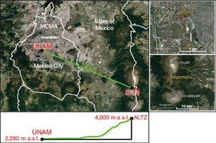
Fig. 1 Location of UNAM station within the Mexico City Metropolitan Area (MCMA) and ALTZ mountain site (top, left), separated by a line-of-sight distance of 60 km (green line); political boundaries of Mexico City and the State of Mexico are shown in white and the altimetry is shown in the lower panel. Right panels show details of the neighboring terrain for UNAM (top) and ALTZ (bottom).
In the top-down approach that combines in situ observations of CO2 concentrations with atmospheric transport models in cities, a critical consideration is the ability of the sampling scheme to discriminate between the regional background level and the local enhancements of CO2 due to fossil fuel usage in the urban area (Turnbull et al., 2014). Coastal locations and remote sites have been traditionally selected for background measurements, since they are representative of the global, well-mixed, marine boundary layer, free from the influence of local sources or sinks of CO2. For a continental city, however, mountain stations at nearby locations may be a better option. Under the adequate meteorological conditions, these sites capture a free-troposphere, regional background signal better suited to interpret patterns of regional exchange (Zhang et al., 2013; Turnbull et al., 2014; Conil et al., 2019). However, city sources and sinks may still influence the background sites (Zellweger et al., 2009; Zhang et al., 2013; Yuan et al., 2019), thus a screening procedure is needed to assure the regional background estimation is free from the signal of the adjacent urban environment.
In this contribution, we present a 5-year time series showing the variability of surface CO2 in central Mexico using high-precision in situ analyzers at two stations, UNAM and Altzomoni, representing urban and background environments. Our main objective is to describe the measurement systems at both sites, examine their performance, and characterize the trend, seasonality and daily cycles on each record. We aim to examine the suitability of the mountain station to monitor regional background conditions, and to evaluate the usefulness of this record to discriminate between the signals of the biogenic exchanges and the anthropogenic enhancement at the urban station.
2. Site description
2.1. The RUOA network
The University Network of Atmospheric Observatories (RUOA, https://ruoa.unam.mx) is comprised of 16 measurement stations within the Mexican territory that provide high-quality data for research and teaching. Six of these stations in both urban and natural settings include high precision GHG analyzers and all of the RUOA stations are fully instrumented to routinely monitor ancillary meteorological variables such as air temperature and relative humidity, wind speed and direction, global solar radiation and barometric pressure, among other atmospheric parameters. The two stations featured in this study, located in central Mexico, are part of this network.
2.2. The urban station
The UNAM atmospheric observatory (19.3262 N, 99.1761 W, 2280 m.a.s.l.) is situated atop of a three-story building on the eastern edge of the UNAM main campus (730 ha), in southwestern Mexico City, 13 km from the city center (Fig. 1). North and west of the observatory, the campus includes low-rise buildings interspersed with lawns and patches of native shrub. To the east, there is a major public transportation hub and a compact, low-rise, highly populated area flanking the campus (Santo Domingo). An urban natural reserve with an area of 237 ha, called Reserva Ecológica del Pedregal de San Ángel (REPSA), spreads to the south and southwest of the observatory and covers a third of the campus area. This reserve represents a relict of the vegetation that covered this portion of the city before its explosive urbanization during the 20th century (Lot and Camarena, 2009). The dominant vegetation type in the REPSA is xerophilous scrub with few interspersed trees, growing on shallow and low-nutrient soil over a basaltic substrate (Rzedowski, 1954). The climate is temperate sub-humid (García, 1988), with summer rains. Daily records of temperature and precipitation are kept by the Meteorological Observatory of the College of Geography of UNAM since 1963 (http://observatoriometeorologico.filos.unam.mx/2016/10/metadatos-historicos). In a period of 57 years, the annual temperature averages 15.6 ºC (min/max range from 14.3 ºC to 17.4 ºC), the temperature peaks at 26.7 ºC on average in May, the warmest month of the year (range 23.2 ºC to 30.9 ºC), and the daily minimum temperature is 3.9 ºC on average in January, the coldest month (range 1.5 ºC to 6.8 ºC). Mean annual precipitation is 870 mm (ranging from 624 mm in 1982 to 1201 mm in 2006), 90% of which falls between May and October. The annual maximum occurs in August and September (~180 mm/month) and the minimum in January, when only 5 mm of total precipitation fall on average. From RUOA hourly records, at a daily scale, wind speed peaks around 17-18 h and the minimum occurs at 5-7 h. Annually, the windiest months are March and April, with daily peak wind speeds of 3.0 ± 1.1 m/s on average, while the daily minimum peak occurs in December, with only 1.9 ± 0.9 m/s on average. The diurnal cycle of wind direction will be discussed in terms of its influence on CO2 mole fraction in subsequent sections.
2.3. The high-altitude station
The Altzomoni (ALTZ) atmospheric observatory (19.1187 N, 98.6552 W, 3985 m.a.s.l.) is located 60 km ESE in a straight line from the UNAM site (Fig. 1), and 48 km at 280º from the city of Puebla (1.5 million inhabitants). The observatory lies in a mountainous pass between the active Popocatépetl volcano to its south, and the dormant Iztaccíhuatl volcano to its north, inside the Izta-Popo-Zoquiapan National Park and Biosphere Reserve (Fig. 1), far from immediate sources of anthropogenic emissions. The immediate surroundings of the observatory are just above the timberline (3,700-3,800 m.a.s.l.) (Beaman, 1962); the vegetation cover consists of subalpine grassland dominated by dense tussock grasses and some scattered individuals of Pinus hartwegii Lindl. Pine trees become more abundant at slightly lower altitudes, and along other conifer species form dense forests in the hillsides of the volcanic ridge. From hourly meteorological records kept by RUOA since 2011, the mean annual temperature is 4.9 ºC (ranging from 4.7 ºC to 5.3 ºC); the warmest month is April, with a daily maximum temperature of 9.7 ºC on average (range from 3.9 ºC to 14.8 ºC), and the coldest month is January, with a daily minimum temperature of -0.1 ºC on average (range from -6.5 ºC to 4.8 ºC). Throughout the year, the diurnal temperature oscillation is moderate (6.1 ± 1.9 ºC). Annual precipitation averages 780 mm (from 573 mm in 2016 to 1052 mm in 2013); on an annual basis, 85% of the rain falls between May and October. June and August are the wettest months of the year (~170 mm/month) while December is the driest, with only 5 mm of average cumulative rain. Daily wind speed peaks at 10 h from October to mid-March at an average of 4.7 ± 2.7 m/s; the maximum shifts to a broader peak around 16 h during March to May, at 4.1 ± 1.7 mean wind speed, and it is displaced to the late evening (20-21 h) for the whole summer (June to September), when the it reaches 5.6 ± 2.7 m/s on average, the highest daily maxima year-round. The weather is also characterized by high levels of global horizontal irradiation (5.0 kWh m-2), and an average of 32 frost events per year. Climate is temperate, semi-cold, sub-humid, with a mild summer (García, 1988).
3. Sampling protocols and instrument calibration
Sampling at the UNAM site of atmospheric mole fractions of CO2, CH4, CO and H2O started on July of 2014, with a Cavity Ring-Down Spectrometer (CRDS) model G2401 from Picarro Inc. Since the beginning of its operation and until July 2019, the air inlet was located on the rooftop of the observatory, at 16 m.a.g.l. The sampling line length from the inlet to the analyzer was under 5 m; air was drawn to the analyzer with an external low-leak diaphragm pump (A0702, Picarro Inc.) and no filtering or air drying system was installed. A calibration system was set up in December 2018, when three 29-liter gas tanks (see Table I), traceable to the WMO X2007 scale for CO2, were acquired from the National Oceanic and Atmospheric Administration Earth System Research Laboratory (NOAA ESRL). Each gas cylinder was equipped with a Scott Q1-14B nickel-plated brass regulator (Air Liquide) and connected to a programmable 8-port rotary valve (EMTSD8MWE, VICI) that selects between gas streams. The sampling line was replaced by a dedicated tubing of ¼” OD (Synflex 1300, Eaton); air drawn from the inlet passes through a 2 μm ceramic filter (FS-2K, M&C TechGroup), a 2 μm sintered filter (SS-2F-2, Swagelok), and then to the rotary valve. Before reaching the an- alyzer, the air is dried using a Nafion membrane (MD-070-144S-4, PermaPure) in ‘reflux mode’: the stream of dried air from the low-pressure exhaust of the analyzer as a purge gas in counter-flow.
Table I Characteristics and site of deployment of calibration standards and target gas cylinders.
| Tank ID | Lab | CO2 (μmol mol-1) | CH4 (nmol mol-1) | CO (μmol mol -1) | Deploymenta | |
| Dec 2018- Aug 2019 | Aug 2019- ongoing | |||||
| CC506424 | NOAA | 391.16 | 1827.25 | unknown | UNA.Cal1 | ALZ.Cal1 |
| CB11619 | NOAA | 405.21 | 1896.25 | unknown | UNA.Cal2 | ALZ.Cal2 |
| CC506485 | NOAA | 420.22 | 1961.20 | unknown | UNA.Cal3 | ALZ.Cal3 |
| D856136 | LSCE | 366.69 | 1721.43 | 222.43 | -- | ALZ.TGT |
a Cal: calibration tank; TGT: target tank.
Prior to installing the Nafion dryer, a single calibration was performed on December 2018 without drying the sample, and the resulting coefficients were retroactively applied to correct all past measurements. Additionally, the sensitivity of the Picarro analyzer to varying levels of humidity in the incoming air stream was tested through the water droplet method (Rella et al., 2013). A 0.2 ml droplet of ultra-pure water (Milli-Q, Millipore) was injected with a syringe directly into the inlet of the CRDS instrument, upstream of the hydrophobic internal filter, in order to humidify the dry gas stream from a gas tank. The wetted internal filter is progressively dried by evaporation with the dry air stream applied, which results in a gas stream with a stable GHG dry mole fraction and a decreasing water vapor content. The procedure was repeated three times and the results used to assess the Picarro built-in correction and to derive analyzer-specific coefficients to correct for the effects of H2O on the GHG dry mole fraction measurement, mainly dilution and spectral line broadening. After these initial tests, a monthly calibration was established.
In March 2019 a second and longer dedicated sample tube was installed at a nearby tower so that the inlet reached 24 m.a.g.l., in order to reduce high-frequency variations from local sources. During a period of about 5 months, the incoming air stream to the analyzer was alternated between the low and high inlet every 15 min; the first 5 min of each period were discarded, and the molar fraction of CO2 was compared between heights. On 23 August 2019 the lower inlet was cancelled; however, given that the measurements done at 24 m comprise a minor portion of the dataset all analysis presented here are based solely on the roof-level data.
In August 2019 the set of NOAA cylinders was replaced by three calibration tanks and one short-term target tank (40 l) provided by LSCE, and calibrated against their NOAA secondary scale (Table I). This set of standards encompass a higher range of molar fractions of CO2 (and CH4) that are better suited for the higher values expected in the urban atmosphere of Mexico City. A target tank which does not participate in the calibration corrections, is measured routinely as a quality control (Laurent, 2017). A final measuring protocol with the target tank alternating with the sampling line and one calibration per month was established (Table II).
Table II Final measurement and calibration scheme for Picarro analyzers on UNAM and ALTZ stations.
| Injection duration (min) | Cycles | Frequency | |
| Calibration standard 1 | 20 | 4 | Monthly |
| Calibration standard 2 | 20 | 4 | Monthly |
| Calibration standard 3 | 20 | 4 | Monthly |
| Short-term target | 20 | 1 | Every 6 h |
| Atmospheric air | 1200 |
A CRDS analyzer (Picarro G2401) was installed at ALTZ on August 2014. On December 2018, a single calibration using the NOAA standards was performed on the analyzer and the resulting coefficients applied to past measurements. The water droplet test described above was also carried out. Initially the gas sampling tube was connected to a glass manifold that extended above the roof of the enclosure and reached a height of aprox. 4 m.a.g.l. The inlet was replaced by a dedicated sampling line of ¼” OD (Synflex 1300, Eaton) at the same height on January 2019; air is drawn by the external diaphragm pump of the CRDS analyzer and passes through a 2 μm ceramic filter (FS-2K, M&C TechGroup) before reaching the analyzer.
On August 2019, a calibration system was set up at ALTZ using the three NOAA calibration standards previously deployed at UNAM (Table I), with an identical valve and filters, and an identical measuring and calibration sequence (Table II). A Nafion dryer is yet to be installed. At this date the UNAM calibration scale was changed with a set of tanks (traceable to WMO-X2007 reference scale) provided by LSCE. Since the measurements made after this change are not used in this study, we do not describe this new scale further.
4. Data processing
4.1 Record filtering, seasonality extraction and trend retrieval
The spectrometers at both locations collect raw data at ~0.3 Hz. The data were averaged and their standard deviation calculated per minute, then per hour. Calibration periods and times affected by any operator’s interference with the instrument were flagged out, which amounted to 4.6% of hours at UNAM and 15.8% at ALTZ. Daily averages were calculated on the filtered datasets. Hourly data were de- trended by subtracting the daily mean from each hourly average in order to estimate diurnal cycles for each station, free of the influence of the seasonal cycle and long-term trend.
To extract the trend and the seasonal features of the evolution of CO2 at each station, the hourly data were filtered to include only nighttime periods representative of background conditions at ALTZ and those under well-developed turbulence conditions at UNAM. We looked for correlations between dry-air CO2 mole fractions and local meteorological conditions (e.g. wind direction, wind speed, temperature), but no clear patterns emerged. The filtering criteria were thus based only on time-of-day and statistical variability.
Seasonal features, peak-to-trough amplitudes, and long-term trends were estimated for each station using the curve fitting described in Thoning et al. (1989) and the Python code made available by NOAA (Thoning, 2018). This fitting procedure finds a function with a number of polynomial terms and a number of harmonics that approximate the long-term trend of the data and the annual cycle, respectively. We used two polynomial terms and four harmonic terms in our function fitting. The residuals were then filtered through two low-pass filters, one short- term (80 days) to smooth the data, and one long-term (667 days) to capture interannual variations not determined by the fitted function. The polynomial portion of the fitted function plus the residuals of the long-term cutoff filter give a trend series that represents the de-seasonalized upward growth of the CO2 con- centration. The first derivative of this trend series constitutes a continuous growth rate series, i.e. the rate of change of the upward trend. The trend was also used to compute a discrete annual growth rate of CO2, defined as the difference between the average CO2 mole fraction for the month of December of any given year and January of the following year, and the average mole fraction recorded during the same pair of months of the preceding year (Dlugokencky and Tans, 2019).
4.2. Uncertainties
The two analyzers installed at UNAM and ALTZ were purchased on 2014 and they were both manufactured by Picarro Inc. at the same period (S/N CFKADS2141 and CFKADS2142). The precision of the two instruments, calculated as the standard deviation of raw data over 1-minute intervals when measuring calibration gases, are equal to 0.03 ppm and 0.024 ppm respectively for UNAM and ALTZ. This is compatible with the precisions calculated for similar instruments deployed at ICOS sites in Europe (Yver Kwok et al., 2021). Unfortunately, the instruments were operated without reference measurements from summer 2014 to December 2018, so we cannot fully characterize the repeatability and drift for this period. Regular measurements of a target gas at UNAM, performed once per day since December 2018, show a very stable repeatability of 0.02 ppm. Monthly calibrations done at UNAM since December 2018 do not indicate a significant drift. We assume that the calibration coefficients established in December 2018 in the two stations had not changed since the summer of 2014. This assumption leads to an increasing uncertainty the further we go back in time. Most G2401 analyzers have a low CO2 drift, but a drift up to 0.1 ppm yr-1 cannot be excluded (Yver Kwok et al., 2015).
It is important to point out that the calibration scale used at UNAM does not cover the full range of measurements, especially the high concentrations observed at night. Indeed, at UNAM, 8% of the daytime observations and 22% of the night time hourly means are above 450 ppm. However, the Picarro G2401 has been evaluated at different laboratories and has exhibited remarkable linearity. Yver Kwok et al. (2015) have tested the same instrument for CO2 concentrations up to 500 ppm, and the NOAA central laboratory uses an earlier version of the same CRDS analyzer (Picarro G2301) to certify calibration material up to 600 ppm (Tans et al., 2017). Both studies show the response of the CRDS instrument to be linear. The results of the linear fit to our sequences of three calibration tanks indicate that the reduced scale does not have an impact on the linearity of the instruments’ response. The residuals of the linear regressions are within a min/max range of -0.02 to +0.04 ppm and -0.02 to +0.03 ppm for UNAM and ALTZ, respectively. The mean RMSE for all instances of the calibrations are 0.01 ppm for UNAM, and 0.02 ppm for ALTZ.
The humidifying technique of the water droplet performed on site allows the evaluation of the built-in factory water vapor correction, and the determination of a new correction, specific to the tested analyzers, with an uncertainty typically around 0.03 ppm for CO2 (Laurent et al., 2019). The built-in factory correction assessment showed an unusual CO2 response to H2O with a residual correction error of -0.22 ± 0.02 ppm and -0.03 ± 0.02 ppm for UNAM and ALTZ respectively, over their site-specific H2O atmospheric range. The residual error of the specific H2O correction determined on site was estimated to be between -0.05 ppm and +0.05 ppm for CO2, depending on the H2O content. Even though the new specific correction seems to improve the performance, it has not been implemented on the database yet, due to our low confidence on the unusual CO2 response to H2O. Indeed, the droplet test must be performed again on site in order to increase this level of confidence. Moreover, the H2O correction resi- dual error may drift over time for CO2. The drift magnitude depends on the H2O content: below +0.01 ppm CO2 per year for H2O lower than 10 000 ppm and up to +0.03 ppm CO2 per year for H2O between 20 000 and 25 000 ppm (Laurent et al., 2019). In consequence, with a H2O content typically below 15 000 ppm at UNAM and 10,000 ppm at ALTZ during the dry season (November to April), the H2O correction drift is not significant (below 0.05 ppm CO2) for either station over the 4-year period preceding the water droplet test (December 2018). During the wet season (May to October), with a H2O content up to 25,000 and 20,000 ppm respectively for UNAM and ALTZ, the H2O correction drift may induce a residual error up to -0.14 and -0.11 ppm of CO2 at these locations, respectively, on the oldest data and highest H2O content. However, based on experience collected by testing more than 50 CRDS analyzers at LSCE (Laurent et al., 2019), the factory water vapor correction assessed on UNAM and ALTZ analyzers does not show a typical drifted response to H2O. At this stage, the overall uncertainty related to the water vapor correction for UNAM and ALTZ is estimated at ±0.2 ppm and ±0.05 ppm CO2, respectively, over the whole period.
5. Results and Discussion
5.1. Daily cycles
The average daily course of CO2 molar fractions at UNAM is presented in Figure 2A, for both weekdays (Monday to Friday) and weekends/holidays. Irrespective of the day of the week, the overall pattern is consistent with a dominant effect of the boundary layer height on the CO2 concentration. A maximum CO2 level is reached daily between 6 and 7 h (all times are LST), then as sun rises and warms the surface, the boundary layer grows and turbulent mixing of the atmosphere increases, as described by García-Franco et al. (2018). The CO2 is diluted over a larger air volume, so its concentration decreases steadily, down to its minimum at 16 h. After sunset, the increase in atmospheric stability reduces the depth of the boundary layer and produces a steady buildup of CO2 during the night in this shallower layer.
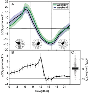
Fig. 2 A) Diurnal cycle of hourly, detrended CO2 measurements at UNAM for weekdays (green) and weekends/holidays (blue). The polar plots inserted show the frequency distribution of wind directions for the periods 0-8 h, 8-16 h, and 16-24 h. B) Mean diurnal difference in CO2 molar fraction sampled at 16 m and 24 m.a.g.l between March 8th and August 23rd, 2019. Error bars are 95% CI. C) Box and whiskers plot of difference in molar fraction between heights. Percentiles shown are the 1st and 99th (crosses), 10th and 90th (cap of whiskers), 25th, 50th and 75th (box). The central black dot indicates the mean.
A further inspection of the prevalent wind direction at different times of the day confirms that the boundary layer dynamics is the main controller of the observed CO2 cycle and offers some insight into the influence of the underlying urban surface. The polar histograms inserted into Figure 2A show a rapid change in the predominant wind direction from the NW quadrant at night (23 - 8 h) to NE-SE sector for most of the day (8 - 15 h), while from 16 h to 23 h the wind directions are more evenly distributed over the NE to WNW sector. The location of the UNAM station is such that the wind coming from the west should carry the signal of the more vegetated surface that releases CO2 at night, while lar- ger emissions could be expected from the more urbanized and almost devoid of vegetation eastern sector during the day. However, the observed daily pattern does not show an association between the relative position of the station and the wind direction, as the concentration falls steadily during the times of the day when the predominant wind comes from the heavily populated sector. The nighttime buildup might include the CO2 respired by the vegetation on the campus side, but the observed enhancement occurs year long and even intensifies in winter, when the vegetation is less active.
In megacities where large anthropogenic emissions dominate, CO2 molar ratio may differ between weekdays and weekends since traffic and other human activities in general diminish noticeably during non-working days. Analyses of surface CO2 records in Melbourne (Coutts et al., 2007), Lecce (Italy) (Contini et al., 2012), Mexico City (Velasco et al., 2014), Helsinki (Kilkki et al., 2015), Sakai (Ueyama and Ando, 2016) Beijing (Cheng et al., 2018) and Chennai (Kumar and Nagendra, 2015), have found perceptible influences of traffic volume on daily concentration and flux patterns. Even in remote marine stations and continental mountain measurements, the weekly periodicity of the anthropogenic activity of nearby cities has been detected and used to unravel the biogenic and anthropogenic contributions to atmospheric CO2 (Cerveny and Coakley, 2002; Yuan et al., 2019). However, it is also common for the daily to seasonal variability of urban environments to be driven by the dynamics of the boundary layer depth, concealing the signal of the human activity, as has been shown in locations like Basel (Schmutz et al., 2016), and in suburban and central London (Hernández-Paniagua et al., 2015; Helfter et al., 2011). At UNAM, we found similar daily cycles of CO2 molar ratio for weekdays and weekends/hol- idays (Fig. 2A). On non-working days, a peak anomaly of ~17 ± 3 ppm with respect to the daily average occurs between 6 and 7 h, while during the weekdays the peak reaches 20 ± 4 ppm. The only noticeable but transient difference between days of the week occurs in this early morning maxima for April and May (not shown), when it reaches 32.6 ± 4.0 ppm above the daily average from Monday to Friday, in contrast to 23 ± 3 ppm during weekends and holidays. On the year-round average, the mean daily amplitude (peak to trough) during weekdays is 45 ± 17 ppm, and 43 ± 18 ppm during non-working days. Weekday and weekend daily courses show considerable overlap, and there are no evident features associated to diurnal changes in traffic volume.
Our analysis indicates that there is a significant positive difference between the roof level measurements and those made 8 m above, for the period between March and August 2019 (mean difference 1.23 ppm, [1.15, 1.37] 95% CI) (Fig. 2B, 2C). This gradient reaches a maximum of 4 ppm at 6 h, coinciding with the largest CO2 accumulation in the stable surface layer before dawn (Fig. 2B). The difference decreases rapidly as the turbulent mixing takes up in the early morning, remains stable until 17 h, and begins to gradually grow again as the sun goes down. On average, between 9 h and 17 h the difference between the two sampling levels is equal to 0.31 ± 0.20 ppm.
At ALTZ, four diurnal cycles in the de-trended CO2 mole fraction can be distinguished as the year progresses (Fig. 3). The periods roughly correspond to dry wintertime (Jan-Mar), dry springtime (Apr-May), rainy season (Jun-Oct) and late fall (Nov-Dec), when some precipitation may still occur. The overall average daily amplitude is 7.2 ± 2.5 ppm; it goes from a minimum of 5.7 ± 2.1 ppm in the dry winter period to a maximum of 8.3 ± 2.3 ppm in the rainy season. From November to May, the daily maximum occurs in the evening, between 18 and 21 h, and the mean concentration continues to decrease the rest of the night. During the rainy season the maximum is displaced to a later period (0-5 h) and the CO2 mole fraction is mostly constant throughout the night. A sharp decrease ensues sunrise, and the minimum is reached from 9 -11 h; slightly earlier in Apr-May (~9 h) and slightly later from June to Dec (~11 h). From June to October the afternoon increase from the minimum CO2 mole fraction is slow up to 16 h, and then increases quickly back to nighttime values.
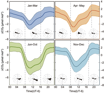
Fig. 3 Diurnal cycles from hourly, detrended CO2 measurements at Altzomoni (ALTZ) for different periods of the year. Inserts are circular histograms of the wind direction for the periods delimited by the light gray vertical lines.
In general, the seasonal changes in daily patterns of surface CO2 at the ALTZ mountain site are consistent with a combination of the aforementioned regional boundary layer dynamics and the local effect of vegetation activity. The tussock grasses in the immediate vicinity of the station and the conifers covering the hillsides of the mountainous range capture and release carbon more actively during the warm, wet season. After the onset of the rains in May, we observe a larger daily amplitude of the CO2 cycle, a more prolonged afternoon minimum, and a larger accumulation at night from June to October, all consistent with increased photosynthetic uptake during the day and increased respiration by vegetation at night. However, a stronger vegetation sink and a more effective vertical mixing of the surface layer are correlated on daily, seasonal and annual basis, so their relative contributions to the daily patterns along the seasons are not easily unraveled.
One interesting feature of the daily cycle of the dry season, is a small but consistent enhancement from midday to the late afternoon (11-16 h). It is more prominent in April and May, and although present during the rainy season, it is considerably shortened (12-15 h). This afternoon enhancement could be the re- sult of a change in local biogenic emissions, the transport of air parcels enriched with anthropogenic CO2 from adjacent cities, or a mixture of these situations. It has been documented that the convective boundary layer starts to develop over Mexico City one hour after sunrise and reaches 2000 m above UNAM’s elevation around midday (Shaw et al., 2007, García-Franco et al. 2018). From January to May, wind from the WNW sector dominate from 0 to 16 h (Fig. 3), consistent with an upslope flow of polluted air masses from the MCMA arriving to ALTZ at midday. In contrast, wind from the E-ESE prevails from June to October; if no recirculation occurs, the smaller increase in CO2 from 12 to 15 h in the rainy season could be the result of lower emissions from Puebla reaching ALTZ, having being partially offset by the photosynthetic uptake of crops and forests as air traversed over the valley and the mountain slope. Granted, the anemometer used in this analysis is situated only at 5 m.a.g.l. at the station, therefore its measurements are likely influenced by the local topography and might not reflect regional circulation. However, the detection of an enhancement of other combustion-related tracers such as CO and NOx at the Altzomoni station during the afternoon is consistent with polluted air parcels being transported from the major neighboring cities (Whiteman et al., 2000; Baumgardner et al., 2009). Preliminary analyses of FTIR solar absorption measurements at Altzomoni show larger CO total columns from January to June, and transient elevated values around 15 h and 18 h in April and May only (N. Taquet, unpublished data).
At the end of the dry season, a contribution from biomass burning to CO2 levels can also be expected from both forest fires and prescribed agricultural burnings, a common practice in the region. However, this alone would not explain the persistence of the daily enrichment well into July and August, in the mid- dle of the rainy season, because most natural and manmade fires take place in March and April, are less frequent in May, and stop after the rains start (Gutiérrez Martínez et al., 2015).
5.2. Seasonal variation and long-term trend
The hourly measurements obtained at UNAM from July 2014 to August 2019 present a large variability (Fig. 4, gray). Once the invalid data -previously defined as calibration periods and times when operator interference occurred- are discarded, the hourly average of CO2 mole fraction ranges from 392 to 577 ppm. The overall mean (± SD) of the original (not de-trended) series is 427.7 ± 16.5 ppm. Values in excess of 450 ppm constitute 17% of the dataset. The average mole fraction are in reasonable agreement with a previous study of flux measurements over a densely populated neighborhood in Mexico City, in which Velasco et al. (2005) found a mixing ratio range of 398 to 444 ppm, and an average of 421 ppm. The slightly higher mean concentration reported here could be attributed to a combination of the CO2 added to the atmosphere between 2003 and 2018 globally (35 ppm) (Dlugokencky and Tans, 2019) and the increase in CO2 emissions that the city has experienced in the years since the Velasco et al. (2005) study took place. The official CO2 annual emissions in 2004 were 35.8 Mt (SEDEMA, 2008) and 52.5 Mt for the year 2016 (SEDEMA, 2018). Additionally, sampling in the earlier study took place during a short, three-week campaign in spring which included Easter week, a holiday period for schools in Mexico (Velasco et al., 2005). Our CO2 levels are comparable to those reported for other megacities like Beijing (Song and Wang, 2012) where monthly averages range from 400 to 440 ppm. Similar concentrations are also observed in Paris, Cité des Sciences, where the CO2 average observed over the same period (2015-2019) equals 426 ppm, with a higher variability in the hourly concentrations, ranging from 388 to 754 ppm (Lian et al., 2019), probably due to a more dynamic atmospheric boundary layer (Pal and Haeffelin, 2015). On the other hand, the short term variability (calculated as the hourly standard deviation of minute averages) is higher at UNAM site (3.6 ppm) compared to Cité des Sciences in Paris (2.0 ppm), which probably reflects a higher exposure to local sources of CO2.
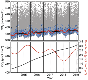
Fig. 4 Above: Hourly (gray) and daily (blue) average of daytime (13-17 h) CO2 mole fractions at UNAM, smoothed fitted function (red) and polynomial component of fitted function (black). Below: trend (black) and growth rate (red) for 2014-2019.
In order to estimate the five-year trend in the UNAM series, we selected only daytime periods from 13 to 17 h, with hourly standard deviations SD < 6 ppm. These filters simultaneously exclude hours when transient and very local effects were recorded (e.g. people working close to the gas intake), and periods when hour-to-hour means differ by more than 3 ppm. Point-like local disturbances are less common at night, but CO2 concentrations steadily rise all night long as the boundary layer stability increases; additionally, nocturnal CO2 exhibits larger effects of seasonality compared to daytime (not shown). We excluded also the observations made at a higher level above ground starting on August 2019. Therefore, the trend, seasonal amplitude, and growth rate were computed for the period between July 2014 and August 2019 only.
The results of fitting NOAA’s CCGCRV function (Thoning et al., 1989) to the filtered dataset at UNAM are also depicted in Figure 4. We estimated an annual growth rate of 2.4 ppm yr-1 for 2014-2019, slightly lower than the global growth rate and the rate reported for Mauna Loa (both 2.6 ppm yr-1) over the same period (Dlugokencky and Tans, 2019; Tans and Keeling, 2019). The continuous growth rate shows a maximum at the end of October 2015 and a minimum at the end of July 2018 (Fig. 4). Our time series is too short to attempt a correlation between the observations and inter-annual climate drivers, but it is worth mentioning that from March 2015 and March 2016, one of the strongest ENSO events on record took place (Chen et al., 2017). In Mexico, the El Niño phase of ENSO is associated with negative precipitation anomalies in the northern and central parts of the country, which can reach deficits of up to 250 mm in the southwestern area of Mexico City, causing increased drought and a higher occurrence of forest fires (Bravo-Cabrera et al., 2018).
A measurement of the evolution of the concentration of CO2 in the atmosphere that is closely related to the annual growth rate is the slope of the polynomial component of the fitted CCGCRV function (Thoning et al., 1989), which we estimated also as 2.4 ± 0.5 ppm yr-1. This value is directly comparable and identical with the yearly gain estimated by Baylon (2017) for total column CO2 at the same site for the year 2016.
The seasonality of data at UNAM is presented in Figure 5. Annual averages were subtracted from daily data to remove the long-term trend from the seasonal change. There is an annual maximum in mid-December, likely due to the shallower boundary layer that prevails during winter (García-Franco et al., 2018), as previously explained. The summer-autumn minimum occurs in mid-September, when both the dilution of trace gases in a deeper convective boundary layer and more active urban vegetation draw down of CO2 occurs. A secondary maximum occurs consistently right before the onset of the rains; we suggest that it is likely not thermally-driven but reflects 1) a significant contribution of transported CO2 from agricultural burnings and forest fires outside the city, which peak at this time of year, and whose effects on air quality in the city’s metropolitan area have been documented elsewhere (i.e. Yokelson et al., 2007; Tzompa-Sosa et al., 2016), and 2) the lack of photosynthetic uptake by vegetation and the dominance of respiration at the end of the dry period. A simultaneous increase in the concentration of other gases and biomass burning tracers in the particulate matter added to the atmosphere during the spring months would lend support to the biogenic origin of these enhancements. Indeed, a preliminary analysis of the CH4 data from the Picarro in our study suggests that minor enrichments do occur in April and May for three out of five years of observations at UNAM (2015-2019). However, in general, the concentration of CH4 in the city is highly variable and it shows large events likely of local origin throughout the year (Bezanilla et al., 2014). A more comprehensive analysis of wind trajectories of the spring enhancements and a concurrent measurement of other biomass burning products is warranted for a more conclusive attribution of emissions to a specific source.
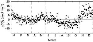
Fig. 5 Average annual course of de-trended daily means of CO2 mole fraction at UNAM for the period 2014-2019.
The daily amplitude shows little seasonality, with a maximum in late fall (50.5 ± 18.9 ppm; Nov-Dec) and a minimum in the dry winter (42.2 ± 14.9 ppm; Jan-Mar), the latter is not significantly different from the rainy season (43.0 ± 18.3 ppm; Jun-Oct) or the dry season average (45.5 ± 14.8 ppm, Apr-May). The average seasonal amplitude was 8.9 ppm, with little interannual variation (8.2 ppm in 2018 to 10.2 ppm in 2015). In the only other long-term CO2 monitoring study in a tropical city that we are aware of, Roth et al. (2017) showed a larger seasonal amplitude of ~14 ppm for Singapore.
Seasonality and trend for ALTZ were computed using only nighttime data (19 to 5 h) and hourly averages with standard deviations lower than 2.0 ppm. The selected daily period is the most appropriate to avoid the influence of either local vegetation activity or polluted air masses from urban areas, and therefore suitable to monitor conditions representative of the free troposphere. The overall mean CO2 mole fraction is 406.2 ± 5.6 ppm, slightly higher than NOAA’s global average for the same period (404.9 ppm). We found an annual average growth rate of 2.6 ppm yr-1 from 2015 to 2019, and again, like at UNAM, the continuous growth rate shows a maximum during the second half of 2015 (Fig. 6). The annual growth rate at ALTZ is in agreement with NOAA’s global rate and Mauna Loa’s (2.6 ppm yr-1), but is slightly higher than the annual growth rate we obtain from NOAA’s data taken at the MEX station in Veracruz (2.4 ppm yr-1) over the same period, at almost the same latitude but further away from the influence of large cities and at a higher altitude. In short times series, however, trend estimates and computations of growth rates are very sensitive to high or low years, so meaningful comparisons are difficult to establish at this point. The slope of the first-degree polynomial of the CCGCRV adjusted curve is 2.7 ± 0.0 ppm yr-1, close to the comparable annual increment derived from the total column measurements for the period 2013-2017 (2.6 ppm yr-1) (Baylon, 2018).
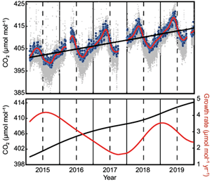
Fig. 6 Above: Hourly (gray) and daily (blue) average of nocturnal (19-5 h) CO2 mole fractions at ALTZ, smoothed fitted function (red) and polynomial component of fitted function (black). Below: trend (black) and growth rate (red) for 2015-2019.
A marked seasonal cycle is discernible with a maximum between the last week of April and the first half of May, and a minimum in the last days of August and the first week of September. The cycle presents an average amplitude of 10.0 ppm, ranging from 8.4 ppm in 2015 to 10.6 ppm in 2018. In order to highlight local contributions to the seasonality of the CO2 annual cycle, we extracted the de-trended monthly means and compared them to the typical seasonal cycle estimated from the reference Marine Boundary Layer (MBL) time series at a latitude of 19º N, for the period 2015-2019 (Fig. 7). The reference MBL record is computed from averages of weekly measurements of several long-lived atmospheric trace gases from the Cooperative Global Air Sampling Network (Conway et al., 1994). A subset of the sites is selected for the CO2 MBL reference; only remote, sea level marine sites that sample well-mixed air from onshore prevailing wind directions are considered. The time series is therefore representative of background conditions of CO2 in the atmosphere.
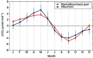
Fig. 7 De-trended, monthly CO2 mole fraction at ALTZ (blue) and from NOAA’s Marine Boundary Layer product for a latitude of 19º N (red), averaged over 2015-2019.
Times of seasonal maximum and minimum concentrations are coincident in both datasets, and in general both curves exhibit considerable overlap, although peak-to-trough seasonal amplitude is lower for the MBL (8.8 ppm), as data from ALTZ shows a slightly higher annual maximum in May probably due to the influence of polluted air masses. From December to February, the atmosphere at ALTZ shows a lower CO2 mole fraction compared to the MBL. Although no systematic observations of photosynthesis by individual species have been carried out at ALTZ, casual observations indicate that the mixture of alpine grassland and conifer forests that surround the station stays more active in late fall and winter than most broad-leaved forests in mid latitudes. The evergreen vegetation would tend to prolong the carbon uptake season compared to species that shed the leaves in the cold season and become dormant, so the differences observed between the MBL signal and ALTZ are likely reflecting the influence of the regional vegetation acting as a sink for atmospheric CO2 during winter.
6. Conclusions
We examined five years of continuous surface CO2 measurements at an urban station in southern Mexico City and at a high-altitude station 60 km away from the first. The daily and weekly variability of the urban site is dominated by the dynamics of the boundary layer depth, with no discernible association to traffic volume patterns or the degree of urbanization of the source area of incoming air. At Altzomoni, the high- altitude station, the daily cycle shows also the influence of the thermally-driven growth of the regional boundary layer, but the effect of the photosynthetic activity of the vegetation controls the features of the cycle throughout seasons, in a pattern consistent with other vegetated surfaces in the northern hemisphere.
The filters applied to the urban record effectively screened out local influences in the immediate vicinity of the air intake, and left only periods of maximum vertical mixing every day. At Altzomoni, the exclusion of daytime values was effective to ensure that trend and seasonality of CO2 concentration were examined under conditions representative of the free troposphere. This background record thus constitutes a suitable baseline to evaluate the evolution of the emissions in the city, as well as the efficacy of mitigation policies. In fact, several features of the regional atmospheric CO2 exchange can only be evaluated as a result of the monitoring of urban and rural sites simultaneously. For example, a daily afternoon CO2 enhancement in Altzomoni’s daily cycle during the dry season signals the effect of polluted air parcels likely coming from Mexico City. Likewise, at UNAM, the CO2 mole fraction of the filtered time series shows an expected maximum in winter but also a secondary peak at the end of the dry season, probably due to incoming emissions from biomass burnings in the agricultural landscape that surrounds the city.
The experimental setup and measurements described here lay the groundwork to the deployment of a network of low-cost CO2 sensors in fifteen stations around the MCMA in the incoming months, in the framework of the Mexico City Regional Carbon Impacts (MERCI-CO2) project. The installation of this network will help in the characterization of the distribution and interplay of sources and sinks of CO2 within the city. It will be complemented by a high-resolution transport model, and by total column CO2 measurements in urban and peri-urban sites. The combined approach will allow the assessment of spatial gradients within, upwind, and downwind the city, and will allow the refinement and verification of current emission inventories.

