


 text new page (beta)
 English (pdf)
 Article in xml format
 Article references
 Send this article by e-mail
 Cited by SciELO
  Similars in
SciELO
Similars in
SciELO 
 Permalink
1. Introduction
The knowledge of boundary layer wind structure in tropical cyclones (TCs) is of great significance for various meteorological and engineering practices, such as path and intensity forecasting of TCs, design of civil engineering structures, and development of wind power projects. In particular, as the design wind loads are proportional to the square of the wind speeds, information of vertical wind speed profiles is of crucial importance for an accurate estimation of wind loads acting on structures.
However, as highlighted by Irwin (2009), the vast majority of building codes still adopt “traditional” models of the atmospheric boundary layer developed in the 1960s. These models are mostly based on observations of synoptic scale systems such as extratropical cyclones and assume a terrain-dependent boundary layer height (gradient height) between 250-550 m. Above the boundary layer top, wind speeds are regarded invariant with height.
Since the 1990s, the deployments of global positioning system (GPS)-based dropsondes by the United States National Oceanic and Atmospheric Administration (NOAA) hurricane research aircraft have provided a wealth of information of TCs in the North Atlantic Ocean. With the aid of high-resolution profile observations, a number of aspects of TCs have been investigated, including air-sea interaction (Powell et al., 2003; D’Asaro et al., 2014), boundary layer height scales (Zhang et al., 2011; Ren et al., 2019), outflow characteristics (Komaromi and Doyle, 2017), inflow angles (Zhang and Uhlhorn, 2012), etc. In particular, composite mean wind profiles measured in the vicinity of TC eyewalls suggest that wind speed increases logarithmically with height in the lowest 200 m, peaks at 500 m, and decreases aloft (Powell et al., 2003; Knupp et al., 2006; Kepert, 2006a, b). It is further found that the height of wind maximum increases with increasing distance from storm center, from around 500 m in the eyewall to 1000 m or beyond in the outer vortex (Franklin et al., 2003; Giammanco et al., 2013). In addition to dropsonde observations, the presence of low-level wind maxima at heights between 500-1000 m is also supported by observations from ground-based remote-sensing instruments (e.g., Donaher et al., 2013; He et al., 2016). Therefore, the assumption in most building codes that wind speed remains constant above the gradient height of 250-550 m may be inappropriate, and an update on these codes may be necessary so as to incorporate the recent research findings and to facilitate structural design of supertall buildings with heights over 300 m.
The South China Sea (SCS) is an ocean basin with frequent occurrence of TCs all-round the year. However, direct meteorological observations of TCs over the SCS are rare. The monitoring of TCs over there is mainly performed using indirect, remote-sensing methods such as geostationary meteorological satellites. There are a limited number of in situ measurements over the sea surface, such as weather buoys, island stations and oil platforms. However, such in situ measurements are very scarce. Starting from 2016, the fixed-wing aircraft of the Government Flying Service of the Hong Kong Government has been equipped with dropsonde facilities, which enable in situ upper air measurements for TCs over SCS. The first complete dropsonde observations of a TC in this ocean has been reported in Chan et al. (2018). Routine meteorological measurements of TCs are conducted since then, and many useful weather data have been collected to support weather forecasting operations and also scientific research. In particular, the vertical wind profiles so collected would be useful to examine the strengthening or weakening of TCs, and to wind engineering applications for updating structural design codes and standards based on actual data.
The abovementioned applications of dropsonde data are studied in this paper, whose major objectives are to investigate the characteristics of inflow and outflow in an intensifying or weakening TC so as to provide references to the intensity forecasting of TCs in weather prediction practices, and to examine whether the wind profiles stipulated in Hong Kong and Chinese wind codes require modification so as to facilitate the TC-resistant design of structures in this region. The present study is novel in the sense that analysis focusing on dropsonde wind profiles has never been conducted before for TCs over the SCS. However, due to limitation of the number of TCs with dropsonde measurements, only four TC cases have been selected in this study. But they are considered to be representative of the typical occurrence scenarios of TCs over the SCS. With the accumulation of more cases, a more systematic and statistical study of TCs using dropsonde data over the SCS would be conducted.
2. Description of the dropsonde system and tropical cyclones
The dropsonde system used in this study is the Airborne Vertical Atmospheric Profiling System (AVAPS) of Vaisala. It has been set up at the two fixed-wing aircraft (Bombardier Challenger) of the Government Flying Service by the Hong Kong Observatory. The aircraft has the major application of conducting search and rescue over the SCS. When there is tropical cyclone over the northern part of the SCS (namely, within the Hong Kong Flight Information Region), the aircraft would be activated to conduct dropsonde measurements, if it has not been engaged in other more urgent tasks.
The flight route of the aircraft is devised and filed to the air traffic management authority in Hong Kong at least three days in advance, based on the predicted track of the tropical cyclone at that moment. It is updated day by day and would be finalized just before the dropsonde flight is conducted. The aircraft would normally fly above the tropical cyclone, at a height of around 10 000 m to release the dropsondes. As agreed with air traffic management authority, only five to 10 launching points would be used in a single mission, which is far less than, for instance, the dropsonde flight performed by the US in the Atlantic Ocean. To ensure data quality, and sometimes to compensate for faulty dropsondes, occasionally up to three or four sondes might be launched at each location in a repeated manner. There are also practical limitations in the timeslots (hour of day) when flight missions can be conducted, which are predominantly in the morning when air traffic is not at its daily peak. Despite these constrains, the dropsonde observation data can provide new insight about the meteorological structures of tropical cyclones over the SCS through previously unavailable in situ profiling measurements. In the present analysis, data of the highest quality from each launching point are selected, where available.
The dropsonde provides horizontal wind, temperature, humidity and pressure from the sea surface up to about 10 km above the sea surface. Wind components are derived from Global Positioning System measurements. The pressure, temperature and humidity data are collected by in situ probe located at the tail end of the dropsonde unit. Wind data are available at up to 4 Hz, while pressure, temperature and humidity measurements are sampled at 2 Hz. In general, it normally takes less than 15 min for the dropsonde to complete the descent from 10 km to the sea surface. Only a limited number of tropical cyclone flights can be conducted every summer because the fixed-wing aircraft could be engaged in other more urgent tasks.
The four selected TCs with dropsonde observations in this paper include tropical storm Aere in 2016, tropical storm Haitang in 2017, typhoon Khanun in 2017, and super typhoon Mangkhut in 2018. Close to the dropsonde observation time, the following information was obtained for each TC:
The intensity of Aere increased from 40 kt (1 kt = 0.5144 m s-1) at 00:00 UTC to 45 kt at 06:00 UTC on October 7, 2016. Dropsondes were released between 01:00-02:00 UTC.
The intensity of Haitang increased from 30 kt at 00:00 UTC to 35 kt at 06:00 UTC on July 29, 2017. Dropsondes were released between 00:00-02:00 UTC.
Khanun, with an intensity of 50 kt at 00:00 UTC on October 14, 2017, exhibited rapid intensification with 10 kt increase in surface wind speed within a 6-h period and reached an intensity of 60 kt at 06:00 UTC. Dropsondes were released between 00:00-02:00 UTC. On the next day (October 15, 2017), the intensity of Khanun decreased from 85 kt at 00:00 UTC to 80 kt at 06:00 UTC. Dropsondes were released between 02:00-03:00 UTC.
The intensity of Mangkhut remained at 100 kt between 09:00 UTC and 12:00 UTC on September 15, 2018. Dropsondes were released between 09:00-10:00 UTC.
To resolve data quality issues, each dropsonde profile has been postprocessed by the Atmospheric Sounding Processing Environment (ASPEN) software (v. 3.4.0) provided by the Earth Observing Laboratory (EOL) with default settings. The quality control process for winds involves hard limit check, outlier check, smoothing using a Cubic B-Spline method (Ooyama, 1987), etc. A detailed description of the quality control algorithms is available at https://ncar.github.io/aspendocs/.
3. Radial and tangential components of the wind profiles
The storm center locations and translational speeds were determined based on the International Best Track Archive for Climate Stewardship (IBTrACS) database (Knapp et al., 2010). A linear interpolation was applied to provide a continuous estimate of the storm center’s location. The dropsonde locations were adjusted to storm-relative coordinates, as shown in Figure 1. Note that open symbols represent dropsonde locations for intensifying TCs (Aere, Haitang, and Khanun on October 14), while filled symbols represent dropsonde locations for non-intensifying or weakening TCs (Khanun on October 15 and Mangkhut). It can be seen that most of the dropsondes were deployed on the left side of the moving storms, where the wind strength is generally lower than the right side. The overwhelming majority of the dropsondes were launched in the outer vortex with distance from the storm center larger than 100 km, while two dropsondes for Aere and two dropsondes for Khanun were released within 100 km from the storm center.
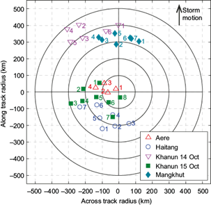
Fig. 1 Strom-relative distribution of dropsonde locations. Storm centre and motion are according to International Best Track Archive for Climate Stewardship (IBTrACS) data (Knapp et al., 2010). Open symbols represent dropsonde locations for intensifying TCs (Aere, Haitang, and Khanun on October 14, 2017), while filled symbols represent dropsonde locations for non-intensifying or weakening TCs (Khanun on October 15, 2017 and Mangkhut). The case number is shown near the symbol for each dropsonde. The storm-relative positions as each dropsonde hits sea surface are shown.
According to the storm-relative locations, the wind speeds were decomposed into radial and tangential components with the storm motion vector subtracted. Note that the horizontal drifts of the dropsondes from the launching points (mostly within 5 km in the radial direction and 20 km in the tangential direction) were considered in the decomposition. The decomposed wind profiles of each TC with subplots stratified by TC quadrant and intensification rate are given in Figures 2 to 5.
The storm intensifying cases are Aere and Haitang, with intensification rates of 5 kt 6 h-1 (Fig. 2), as well as Khanun on October 14 with intensification rate of 10 kt 6 h-1 (Fig. 3). As expected for a TC over the Northern Hemisphere, the tangential components are all anticlockwise. In the Aere cases, there is neither marked inflow or outflow except for case 1 near the storm center. It is speculated that the vertical wind profiles of Aere are twisted by the environmental wind shear. The actual inflow directions would need to be further analyzed by considering the large scale (synoptic scale) atmospheric flow at the time. The inflow layer depth of Haitang is generally around 2 km in the left-rear quadrant, which is somewhat smaller than the height of the maximum tangential wind speed about 5 km. However, in the right-rear quadrant, the inflow is not significant. In some cases (6 and 7), there is neither marked inflow nor outflow between 2-9 km, while in other cases the outflow layer spreads above 2 km. Khanun, which underwent rapid intensification on October 14, features a deep inflow layer. The inflow layer depth generally exceeds 7 km, significantly larger than the height of the maximum tangential wind speed around 1.5 km.
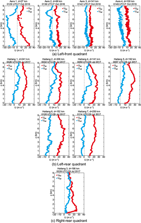
Fig. 2 Wind profiles of intensifying TCs with intensification rate of 5 kt 6 h-1, including Aere on October 7, 2016 and Haitang on July 29, 2017. Utan (red circle): tangential component of wind speed, counterclockwise positive; Urad (blue circle): radial component of wind speed, away from center positive; d: distance from storm center. The case number is shown after the TC name in the title of each subfigure, e.g., Aere 1 represents case 1 of Aere.
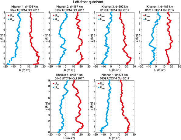
Fig. 3 Wind profiles of an intensifying TC with intensification rate of 10 kt 6 h-1, namely Khanun on October 14, 2017. Nomenclature as in Figure 2.
The mature storm case is Mangkhut with wind strength remaining at 100 kt (Fig. 4). Strong inflow with radial wind speed at 20 m s-1 at a height of 300 m was observed in most cases. Weak outflow was found between 4-9 km. The inflow layer depth around 2 km is comparable with the height of the maximum tangential wind speed. The observed strong inflow may be attributed to concentric eyewalls of the storm (He et al., 2020).
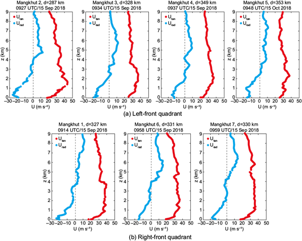
Fig. 4 Wind profiles of a a TC with wind strength remaining unchanged, namely Mangkhut on September 15, 2018. Nomenclature as in Figure 2.
The only storm weakening case is Khanun on October 15 (Fig. 5). The height of the maximum tangential wind speed is around 1-2 km. Shallow inflow layer was observed in the left-front quadrant. While there is an inflow layer in the inner region (case 8), it could be seen that basically there is no inflow within the lowest 4 km in the outer region. There is even outflow in that region. At higher altitudes between 4-9 km, a weak inflow was observed.
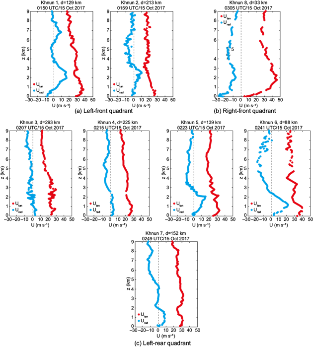
Fig. 5 Wind profiles of a weakening TC at a rate of 5 kt 6 h-1, namely Khanun on October 15, 2017. Nomenclature as in Figure 2.
Based on the above observations, it is indicated that the radial component has inflow at certain sectors of an intensifying TC, particularly in the left-front and left-rear quadrants and over the lowest 2 km. But for a weakening TC, despite an inflow layer in the inner region, basically there is no or little inflow in the outer region. Therefore, a strong inflow may be a precursor of intensification of TCs, while a TC with no or little inflow may not intensify or even weaken. More wind profile samples would need to be analyzed to see if this is a general case.
4. Fitting of vertical wind profiles
Six wind profile models of interest in meteorological and engineering applications are selected for fitting the observed vertical wind profiles. A brief introduction of these models is given below.
The empirical power law is currently adopted by many structural design codes and standards, e.g., Hong Kong (Buildings Department, 2019), China (GB50009-2012, 2012), Japan (AIJ, 2015), and the USA (ASCE, 2016), due to its simplicity. It is expressed as:
where U is wind speed at height z, U ref is the wind speed at reference height z ref (usually taken as 10 m), and α is the power exponent.
The logarithmic law, derived by the Monin-Obukhov Similarity Theory or Mixing-Length Theory, is widely accepted by the micrometeorology community. It is given as:
where κ is the von Karman constant assumed to be 0.4, u* is the friction velocity, and z 0 is the surface roughness length.
As the power law and logarithmic law may be invalid beyond the surface layer, which is generally the lowest 10% of the atmospheric boundary layer, Deaves and Harris (1978) developed an empirical boundary layer wind profile model by matching the surface winds with the geostrophic (gradient) winds (hereafter D-H model). It was adopted by the Australian/New Zealand structural design standard (AS-NZS, 2011) and the Engineering Science Data Unit (ESDU, 1982), and widely utilized in wind engineering applications. The D-H model is expressed as:
where z h is the boundary layer height, empirically determined Eq. (4):
where f is the Coriolis parameter equal to 5 × 10⁻⁵ s-1 for latitude 20º.
Likewise, Gryning et al. (2007)) proposed the following wind profile model to simulate the entire atmospheric boundary layer based on the Mixing-Length Theory (hereafter Gryning model):
where l m is the length scale in the middle layer, empirically determined by:
Considering that the hurricane boundary layer may deviate much from non-hurricane boundary layer, Vickery et al. (2009) proposed an empirical wind profile model based on hurricane wind profile observations over the Atlantic Ocean (hereafter Vickery model):
where a = 0.4, n = 2.0, and H* is the boundary layer height parameter, which is allowed to vary with each vertical wind profile.
Recently, Snaiki and Wu (2018) proposed a semi-empirical wind profile model for the hurricane boundary layer (hereafter S-W model):
where η 0 = 9.026 and δ is the height of maximum wind to be fitted.
It is noted that the D-H model and the Gryning model were developed for synoptic scale winds (e.g., extratropical cyclones), and the Vickery model and the S-W model were built based on observations of hurricanes over the Atlantic Ocean. It is therefore of interest to see whether these models are applicable to TC wind profiles over the SCS. It is also meaningful to examine whether these models give a better representation of observed wind profiles than the logarithmic law or power law, which is widely adopted in structural design codes. Specifically, in Hong Kong and Chinese codes, wind speed is regarded to follow the empirical power law below the gradient height (h g ), and be invariant with height above h g , as follows:
where h g is the gradient height (300 m for open terrain in Chinese code, 500 m for Hong Kong code), U g is the design wind speed at h g , and α is the power exponent (0.12 for open terrain in Chinese code, 0.11 for Hong Kong code). The design wind speed is based on extreme value analysis of long-term near-surface wind records from meteorological stations, e.g., in Hong Kong wind code, the design hourly mean wind speed at 500 m is 59.5 m s-1.
However, it is noted that a dropsonde samples the instantaneous features of a TC at a certain storm-relative position. Such instantaneous wind profiles may deviate from wind codes and standards, where a mean wind speed profile associated with a long averaging time period of 10 min (Chinese code) or 1 h (Hong Kong code) is used for design purposes. To diminish such uncertainties, composite wind profiles are examined herein following the approaches by Vickery et al. (2009). The advantage of this technique is that the turbulence features are filtered out, and the composite mean wind profiles are relatively robust so that meaningful information for engineering applications can be retrieved. In the present study, considering that mean wind structures are fairly comparable at similar radii for a certain TC, the wind profiles are firstly grouped by TCs, then further stratified by the distance from the storm center. For Haitang and Khanun on October 14, and Mangkhut, the dropsondes are distributed at similar radii in the outer vortex and thus not further stratified. For Aere and Khanun on October 15, the dropsondes are further stratified into two regimes, one near the eyewall (20-100 km) and the other in the outer vortex (>100 km). Aere outer vortex wind profiles are excluded from the analysis due to data quality issues. Note that while outer vortex wind profiles are investigated in a composite sense, eyewall wind profiles are still examined on an individual basis, considering that their number is rather limited (only two for Aere and two for Khanun on October 15).
Parameters involved in the aforementioned six models, including the friction velocity (u*), roughness length (z 0 ), power exponent in the power law (α), boundary layer height parameter in the Vickery model (H*), and height of the maximum wind in the S-W model (δ), are estimated through least-square fits. Two height ranges of interest to wind engineering were chosen for fitting, namely 10-200 m (low-rise building and wind turbine relevant height) and 10-1000 m (tall building relevant height). To quantitatively evaluate the performances of the six wind profile models in reproducing the observed profiles, correlation coefficient (r) and root mean square error (RMSE) were calculated, as follows:
where y i and x i are the observed and modelled wind speeds, respectively, and n is the sample size.
The fitting results of the wind profiles are shown in Figures 6 to 8, and the corresponding goodness-of-fit statistics are listed in Tables I to III. As suggested by Figure 6 and Table I, all the composite mean wind profiles in TC outer vortex show a logarithmic decay of wind speed with height over 10-200 m, which agrees with Powell et al. (2003), Tse et al. (2013), etc. While the fitted roughness length z 0 for Haitang and Mangkhut is in the order of 10-4-10-2 m and comparable with previous research (e.g., Powell et al., 2003; Donelan et al., 2004), fitted z 0 for Khanun is unusually small (in the order of 10-9-10-6 m). This phenomenon deserves further research. There is little difference between the performances of the six wind profile models in describing the observed wind profiles in terms of correlation coefficient and RMSE.
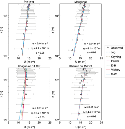
Fig. 6 Composite mean wind profiles over 10-200 m for outer vortex cases, along with model fitting (in logarithmic scale). Dashed lines represent meteorological models (logarithmic law and Gryning model), while solid lines and dotted lines represent engineering models (power law, and D-H, Vickery, and S-W models). Error bars stand for one standard deviation from the mean.
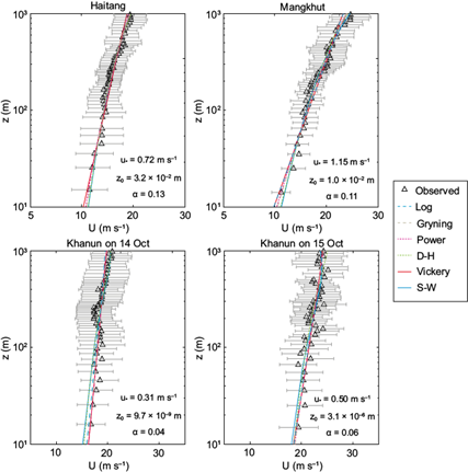
Fig. 7 Composite mean wind profiles over 10-1000 m for outer vortex cases, along with model fitting (in logarithmic scale). Nomenclature as in Figure 6.
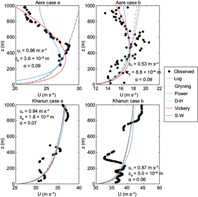
Fig. 8 Instantaneous wind profiles over 10-1000 m for eyewall cases, along with model fitting (in linear scale). Nomenclature as in Figure 6.
Table I Goodness of fit of the models in predicting outer vortex wind profiles over 10-200 m.
| TC | Log | Gryning | Power | D-H | Vickery | S-W | |
| Correlation coefficient r | Haitang | 0.931 | 0.930 | 0.932 | 0.928 | 0.931 | 0.937 |
| Mangkhut | 0.966 | 0.965 | 0.964 | 0.962 | 0.967 | 0.964 | |
| Khanun on October 14 | 0.689 | 0.689 | 0.685 | 0.652 | 0.799 | 0.739 | |
| Khanun on October 15 | 0.765 | 0.766 | 0.765 | 0.766 | 0.765 | 0.766 | |
| RMSE (m s-1) | Haitang | 0.387 | 0.388 | 0.383 | 0.394 | 0.387 | 0.370 |
| Mangkhut | 0.434 | 0.443 | 0.446 | 0.460 | 0.428 | 0.451 | |
| Khanun on October 14 | 0.540 | 0.541 | 0.504 | 0.678 | 0.416 | 0.781 | |
| Khanun on October 15 | 0.951 | 0.950 | 0.952 | 0.950 | 0.951 | 0.949 |
Figure 7 and Table II show the fitting results of TC outer vortex wind profiles over 10-1000 m. It is observed that the logarithmic regime extends up to 1000 m, although the slope of the profile (therefore the fitted z 0 ) may differ from that in the near-surface levels lower than 200 m. This agrees with radar observations of TC stratiform rainbands over land by Donaher et al. (2013). Low-level wind maxima below 1000 m are not captured in these profiles, and there is no evidence that the Vickery or S-W models perform better than the other models. It is noteworthy that wind speed does not remain unchanged above h g of 250-550 m, which disagrees with stipulations in most building codes.
Table II Goodness of fit of the models in predicting outer vortex wind profiles over 101000 m.
| TC | Log | Gryning | Power | D-H | Vickery | S-W | |
| Correlation coefficient r | Haitang | 0.948 | 0.975 | 0.968 | 0.981 | 0.948 | 0.980 |
| Mangkhut | 0.962 | 0.978 | 0.976 | 0.983 | 0.962 | 0.984 | |
| Khanun on October 14 | 0.774 | 0.779 | 0.783 | 0.810 | 0.774 | 0.786 | |
| Khanun on October 15 | 0.843 | 0.841 | 0.841 | 0.826 | 0.845 | 0.844 | |
| RMSE (m s-1) | Haitang | 0.650 | 0.450 | 0.510 | 0.397 | 0.650 | 0.408 |
| Mangkhut | 0.870 | 0.660 | 0.696 | 0.583 | 0.870 | 0.561 | |
| Khanun on October 14 | 0.670 | 0.666 | 0.658 | 0.787 | 0.670 | 0.850 | |
| Khanun on October 15 | 0.848 | 0.854 | 0.852 | 0.941 | 0.843 | 0.877 |
Eyewall wind profiles over 10-1000 m are depicted in Figure 8, and the goodness-of-fit statistics are shown in Table III. It is found that in Aere’s eyewall, the wind speed increases logarithmically up to a height of 500 m, followed by a decrease until 1000 m. The Vickery and S-W models outperform the other four models in depicting this jet-like feature, especially for case a (see upper left panel in Fig. 8), where only the Vickery and S-W models yield positive correlation coefficients. However, in Khanun’s eyewall, jet-like features are not found in the lowest 1000 m. Wind speed generally increases with height despite the presence of some small-scale fluctuations. There is no significant difference between the goodness-of-fit of the six profile models in Khanun eyewall cases.
Table III Goodness of fit of the models in predicting eyewall wind profiles over 10-1000 m.
| TC | Log | Gryning | Power | D-H | Vickery | S-W | |
| Correlation coefficient r | Aere case a | -0.848 | -0.867 | -0.856 | -0.869 | 0.946 | 0.950 |
| Aere case b | 0.295 | 0.266 | 0.282 | 0.288 | 0.594 | 0.548 | |
| Khanun case a | 0.882 | 0.897 | 0.891 | 0.911 | 0.882 | 0.900 | |
| Khanun case b | 0.631 | 0.656 | 0.645 | 0.700 | 0.630 | 0.567 | |
| RMSE (m s-1) | Aere case a | 3.257 | 3.342 | 3.297 | 3.356 | 0.816 | 1.477 |
| Aere case b | 1.688 | 1.810 | 1.751 | 1.788 | 1.323 | 1.375 | |
| Khanun case a | 1.220 | 1.140 | 1.175 | 1.062 | 1.238 | 1.126 | |
| Khanun case b | 2.633 | 2.566 | 2.594 | 2.430 | 2.634 | 2.871 |
it is unclear which are these cases
Overall, the presence of the logarithmic layer in the lowest 200 m of TC boundary layer is relatively robust. But at higher altitudes over 500 m, the wind speed either continues to increase logarithmically or decreases in conformity with the Vickery or S-W models. This contradicts the assumption in most wind codes that wind speed remains constant above the gradient height of 250-550 m. As the overwhelming majority of engineering structures are situated within the lowest 200 m of the atmospheric boundary layer, the application of the simple power law for estimating the design wind loads on them may still be justifiable. However, with the emergence of supertall buildings in the south China coastal region, such as the Ping-An Finance Centre with a height of 600 m (Li et al., 2018), there is a need to improve the wind codes to incorporate the updated knowledge of TC wind profiles, since an underestimation of wind speed may lead to unsafe design and building damages, while an overestimation may result in overdesign and unnecessary cost.
5. Uncertainty analysis
Various uncertainties exist in the analysis of dropsonde wind profiles. The first source of uncertainty is the location of the TC center. This may influence the decomposition of winds into radial and tangential components, as decomposed winds can be quite sensitive to small errors in storm center locations (Ryglicki and Hodyss, 2016; Komaromi and Doyle, 2017). After intercomparing the TC center information provided by several agencies including HKO, CMA, JMA, and JTWC, it is found that the difference is generally within 0.1 degree in both latitude and longitude, suggesting an uncertainty of 15 km in the center position. This has little influence (less than 10% error) on wind profiles in the outer vortex but may largely affect the accuracy of wind decomposition for dropsondes near the TC center, such as eyewall dropsondes in Aere and Khanun, where the error in radial wind speed may be as large as 5-10 m s-1. Another concern is that the TC center may be twisted by the environmental wind shear. However, as information of TC center location as a function of height is not available, a fixed TC center location based on linear interpolation of three-hourly IBTrACS data is still used in the present study.
The second source of uncertainty arises from the horizontal drifts of the dropsondes. The dropsonde follows a Lagrangian trajectory and may drift both tangentially and radially relative to the storm center while descending. In the present study, the drift distances of the dropsondes are mostly within 20 km in the tangential direction and 5 km in the radial direction. The drifts of dropsondes in the radial direction towards the surface wind maximum may lead to stronger reported winds and weaker vertical wind shear near the surface (Powell et al., 2003), and the near-surface portion of the dropsonde profile may depart from what would be anticipated below the upper portion of the profile (Zhang et al., 2018).
The final source of uncertainty is the instantaneous nature of dropsonde measurements. The dropsonde samples the instantaneous features of winds in the turbulent TC boundary layer, therefore dropsonde profiles should be considered as single realizations of winds (Zhang et al., 2018). Consider a turbulence ratio (σ u /u*) of 2.5, the standard deviation of wind speed (σ u ) is estimated to be 1-3 m s-1, implying an inherent departure of ± 1-3 m s-1 from the mean for a single dropsonde wind profile. More cases would need to be accumulated to facilitate a more comprehensive and statistical analysis.
6. Conclusions
The vertical wind profiles of selected TCs over the SCS are studied for the first time using dropsonde measurements. This study could not be undertaken before the introduction of operational dropsonde reconnaissance by the Hong Kong Observatory to the SCS in late 2016. Two aspects of TCs are studied here. First, the strengthening and weakening trends of TCs are analyzed using the radial wind profiles from the dropsonde measurements. It is found that, for TCs strengthening during the time of the measurement, inflow is mostly observed from the dropsonde data, particularly over the lowest 2 km. On the other hand, if the TC weakens, despite an inflow layer in the inner region, the outflow layer widely spreads in the outer region. More wind profile samples would need to be analyzed to see if this is a general case.
Secondly, for wind engineering applications, the vertical wind profiles are fitted using a number of commonly used wind profiles in meteorological and engineering studies. The correlation coefficient and RMSE are calculated to examine the goodness-of-fit of these models. The presence of the logarithmic layer in the lowest 200 m of TC boundary layer is relatively robust. But at higher altitudes over 500 m, the wind speed either continues to increase logarithmically, or decreases in conformity with the Vickery or S-W models, which contradicts the assumption of constant wind speed above gradient height in most wind codes. Since an underestimation of wind speed may lead to unsafe design and building damages, while an overestimation may result in overdesign and unnecessary cost, the observed variation of wind speed above gradient height would have important implications to structural design of supertall buildings in this region, which is prone to the destructive effects of typhoons.
The number of tropical cyclone cases in this study is limited. Yet the results have new insights for tropical cyclones over the SCS, where dropsonde data are being collected every summer. More samples will be collected in the future, and a larger-scale study based on much more tropical cyclones will be performed for a statistical analysis.

