


 text new page (beta)
 English (pdf)
 Article in xml format
 Article references
 Send this article by e-mail
 Cited by SciELO
  Similars in
SciELO
Similars in
SciELO 
 Permalink
1. Introduction
Rice is a major food crop which is grown intensively in India, where it occupies 24% of the gross cropped area and 42% of the total food grain production (Ghose et al., 2013). The lowland rice area in India is about 14.4 million hectares, which represents 32.4% of the total rice area (Singh, 2009). The tropical lowland irrigated rice ecosystem differs greatly from other upland based crop ecosystems, since a continuous water layer is maintained above the soil surface, which strongly influences the surface energy balance components (Tsai et al., 2007; Alberto et al., 2011). Such differential nature of rice cultivation may alter the surface runoff, groundwater storage, water cycle, surface energy budget, and possibly microclimate of the region (Simmonds et al., 1999). The energy balance closure (EBC) in a particular site varied with time and is connected to the quantity of water (Reed et al., 2018). The main storage components for lowland rice are heat stored in standing water, photosynthesis and the soil layer (Tsai et al., 2007). Photosynthetic heat storage and standing water stored contributed about 2 and 0.4% of the available heat flux, respectively (Tsai et al., 2007).
The increase in productivity is the prime goal of an agricultural researcher with an objective to address the food demand of the ever-increasing population. However, the productivity of an agroecosystem strongly responds to all climatic variables, such as atmospheric temperature, precipitation, humidity, solar radiation, and photosynthetically active radiation (PAR). The dynamics of heat fluxes are determined by the nature and type of the vegetation that covers the soil; hence, determining a correct energy balance mechanism is a crucial prerequisite to understand and model an agroecosystem and its interaction with the climatic variables, which is associated with crop yield (Castellvi et al., 2008; Bormann, 2011; Chatterjee et al., 2019a). Surface energy balance is mainly determined by four types of energy fluxes coming into or going out from the surface, i.e., net radiation flux (Rn), sensible heat flux (H), latent heat flux (LE), and soil heat flux (G). H is directed away from the surface throughout daytime, while it is in opposite direction during the evening and nighttime. LE is the consequence of evaporation and evapotranspiration at the surface. Rn is an outcome of radiation balance at the surface, a product of upwelling and downwelling radiations. During daytime, Rn is directed towards the surface of the soil while vice-versa at nighttime. G was different at the surface level than in deeper layers of the soil and had a better closure (Masseroni et al., 2012, 2015; Yao et al., 2008). In principle, an accurate closure leads to the available energy of an ecosystem balancing the energy involved in various processes. Also, this principle includes energy storage terms such as stored energy of net ecosystem exchange and soil heat storage term (Shuttleworth, 2012), heat stored in the soil and water (Meyers and Hollinger 2004), or advection (Heusinkveld et al., 2004). As the different terms of the energy balance cannot be measured fully and correctly, there is an energy balance closure gap in the measured energy balance.
With this view, several studies on the measurements of these components had already been accomplished throughout the world with varying geographical distributions (Campbell et al., 2001; Gao et al., 2003; Yoshimoto et al., 2005; Tsai et al., 2007). However, in India rice cultivation in wet and dry seasons in a tropical lowland ecology has not been sufficiently addressed in a comprehensive study. The two major objectives of this study are: (1) evaluating EB components in a lowland rice paddy, which can be used for meteorological models, and (2) evaluating the closure of surface energy by integrating energy exchange components between the rice and atmosphere.
2. Materials and methods
2.1 Description of the study site and crop establishment
This experiment was conducted at the eddy covariance (EC) system installation site of the National Rice Research Institute (NRRI) in Cuttack, Odisha, India (20º 26’ 60.0’’ N, 85º 56’ 10.9’’ E). The soil at the study site was characterized as Aeric Endoaquept. The texture of the soil was sandy clay loam with bulk density of 1.41-1.43 Mg m-3. The pH (1:2.5 soil:water ratio) of the soil was acidic in nature (6.21-6.32) with no problem of extreme salt concentration as characterized by a low (< 4.0 dS m-1) electrical conductivity value of 0.42-0.45 dS m-1. The total carbon and total nitrogen were recorded in the range of 11.2-11.4 and 0.8-0.9 g kg-1, respectively. The annual recorded precipitation was 1311.90 and 1343.40 mm in 2015 and 2016, respectively. The highest precipitation in both years occurred from June to September, as this period coincides with the monsoon season. The annual average temperature ranged from 22.6 to 31.8 ºC in 2015, and 22.3 to 31.6 ºC in 2016.
The experiment was conducted during the years 2015 and 2016, which have been classified into four categories: dry season (DS, 1-125 Julian days), dry fallow (DF, 126-181 Julian days), wet season (WS, 182-324 Julian days), and wet fallow (WF, 325-365 Julian days). Two rice cultivars (Naveen in the DS and Swarna sub 1 in the WS) were transplanted at the study site in both years at a distance of 20 (row to row) × 15 cm (plant to plant) during January in the DS and July in the WS. The rice was harvested during May in the DS and November in the WS. An average 8-cm standing water was maintained in the experimental field; whenever it reached 4 cm, irrigation was initiated. This practice was continued throughout the seasons up to two weeks before harvest. Fertilizer was applied based on the local recommendation at three stages, viz. field preparation, maximum tillering (MT) and panicle initiation (PI). Compost was applied at a rate of 5 t ha-1 in June during the field preparation for WS rice.
2.2 Instrumentation of the eddy covariance system and data processing
The EC system was established in the center of a paddy field of around 2.25 ha at a 1.5-m height from the ground surface. The measured parameters include H, LE, Rn, G, air temperature (Ta), wind speed, wind direction, and net ecosystem exchange of carbon dioxide (NEE). The H and LE were measured with a fast response three-axis sonic anemometer (CSAT3, M/s Campbell Scientific, Logan, Utah, USA) and open-path infrared gas analyzer (LI-7500, M/s LICOR, Canada). Ta and relative humidity (RH) were recorded using a temperature-humidity sensor (HMP45C, Campbell Scientific) on a half-hourly basis (Campbell Scientific, 2009). The net radiation was measured with a 4-component radiation sensor (CNR4, KIPP and ZONEN, Netherlands). Soil heat flux (G) was measured using soil heat flux plates (HFT3, M/s Campbell Scientific). Soil temperature at 5 and 15 cm soil depth was recorded with a soil temperature probe (107 B, Campbell Scientific). PAR was measured with a PAR sensor (LI190SB). An open path infrared gas analyzer (LI-7500, LICOR) was used to measure NEE (LICOR, 2011). All signals for the sensors were recorded at a sampling rate of 10 Hz and stored in a data logger (CR3000, Campbell Scientific).
EC flux data were processed following Mauder and Foken (2011). The collected EC data underwent flux corrections (Mauder et al., 2006). All other corrections, like time lag (Goulden et al., 1996), frequency response losses (Aubinet et al., 2000), coordinate rotation (Kaimal and Finnigan, 1994) and Webb-Pearman-Leuning (WPL) correction (Burba and Anderson, 2010) were conducted using the EdiRe software. Spikes in data were eliminated by standard procedure (Vickers and Mahrt, 1997; Reichstein et al., 2005). Missing and rejected data was filled up with a “look-up” table approach (Falge et al., 2001).
2.3 Basic theory of energy balance equations
The surface energy budget, which is based on the conservation of energy, can be expressed as the sum of surface LE and H flux equivalent to all other energy sinks and sources (Wilson et al., 2002; Tsai et al., 2007).
where V is the available heat flux at the surface; Rn is the net radiation, calculated using Eq. (2); G is the soil heat flux; S is the heat storage in a layer of soil having a boundary between the soil surface and the plane of insertion of the soil heat flux sensors (Tsuang, 2005; Eq. 3); W is the heat storage in the standing water, calculated with Eq. (4). About 4-8 cm of standing water was maintained throughout the cropping season. Water temperature was calculated indirectly from air temperature following Pakoktom et al. (2014). C is the heat storage in canopy (Garratt, 1992; Eq. 5); F is the photosynthetic energy flux (Eq. 6); LE c is the latent heat flux at the canopy height; H c is the sensible heat flux at the canopy height; H is the surface sensible heat flux, and LE is the surface latent heat flux.
where Rsd is the shortwave downwelling radiation; Rsu is the shortwave upwelling radiation; Rld is the longwave downwelling radiation; Rlu is the longwave upwelling radiation; ρ g , ρ a , and ρ w are the density of the soil, air, and water, respectively; C g , C w and C p are the specific heat capacity of wet soil, water and air, respectively; Z g and Z w are the depth from surface to the point where the soil heat flux sensor was inserted and the depth of standing water in the rice field, respectively; T g and T w are the temperature of soil and water, respectively; H c is the height of EC system (1.5 m); L υ is the latent heat of vaporization; θ is the potential temperature, defined as the potential temperature of an air parcel if it could be transported adiabatically to the surface pressure; q is specific humidity, which may be defined as a mass of water vapor in a unit mass of moist air; is the energy (422 kJ g mol−1) needed to fix one mol of CO2 by photosynthesis (Nobel, 1999); is the molecular weight of CO2, and is the flux of CO2 measured in the EC system. H c and LE c were estimated by Eqs. (7) and (8) as follows (Garratt, 1992):
where the second and third terms on the right are storage and local advected heat fluxes between the height hc and the surface, respectively. Terms u and υ are wind components at x and y direction. Bowen ratio, which was obtained by the H:LE ratio (Tsai et al., 2010), gives an idea of the relative dominance of sensible and latent heat fluxes:
2.4 Analysis of the energy balance closure
In this study, EBC is examined in three ways. The ordinary least squares (OLS) relationship was established between turbulence heat flux (LE + H) and available heat flux (V), which is Rn - G, and linear regression coefficients (slope and intercept) were derived (Wohlfahrt and Widmoser, 2013). Available energy (V) represents the energy left for turbulent heat transfer. This is basically the difference between net radiation and soil heat flux (Gao et al., 2003). This is considered effective assuming there are no random errors in the independent variable, and it can be expressed as:
where a and b are the slope and intercept of the linear regression, respectively. The perfect closure is achieved when the intercept is zero and the slope is 1. Different storage terms like S, W, F, and C are also used as correction in the OLS relationship to get better closure.
EBR can also be used to evaluate the closure (Wilson et al., 2002), which can be expressed as the ratio of cumulative turbulence heat fluxes (LE + H) and available heat flux (V) over a time period:
With the standard EBR values (Eq. 11, EBR I) different storage terms (S, W, F, and C) were used as a correction to get more precise EBR values (EBR II, III and IV).
Residual heat flux (RHF) quantifies the inconsistency between the V and turbulence heat flux (LE + H), and provides information about whether the LE + H measured by the EC system is overestimated or underestimated. This evaluates the degree of EBC achieved (Cava et al., 2008; Wohlfahrt and Widmoser, 2013).
RHF should be zero when the surface energy budget is closed. If RHF is greater than zero, then the supply of energy is larger than the loss of energy; else, the result is the reverse.
3. Results
3.1 Temperature, precipitation and wind characteristics of the site
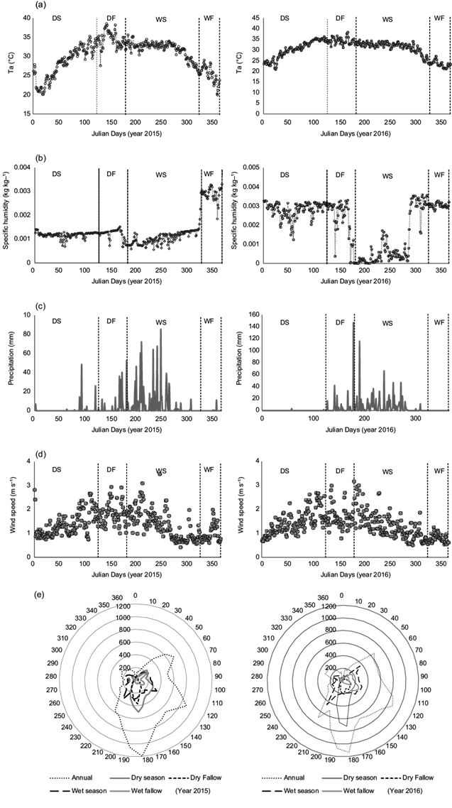
Air temperature varied between 20.1-35.3, 27.6-38.5, 25.6-35.6, and 20.0-29.0 during DS, DF, WS and WF, respectively, in 2015 (Fig. 1a). Similarly, air temperature varied between 20.8-35.5, 31.2-38.3, 23.2-34.7, and 21.0-27.0 during DS, DF, WS and WF, respectively, in 2016. Lower specific humidity (kg kg-1) was observed in DS and DF compared to WS and WF in both years; however, it was much lower in WS during 2016 compared to WS during 2015 (Fig. 1b). Precipitation is well distributed throughout the season except for a few months in DS during 2015 (Fig. 1c); nevertheless, it was more concentrated during DF and WS in 2016. Precipitation in DS amounted to 116.6 mm in 2015, while it was only 4.8 mm in 2016. The highest precipitation was recorded during WS (937.6 and 945.3 mm in 2015 and 2016, respectively), followed by DF (245.3 and 365.6 mm in 2015 and 2016, respectively). The lowest precipitation was recorded in WF (12.4 and 0 mm in 2015 and 2016, respectively). The average wind speed on the site was 1.38, 1.82, 1.38, and 0.98 m s-1 in DS, DF, WS, and WF, respectively, during 2015, while it was 1.46, 1.70, 1.31, and 0.79 m s-1 in DS, DF, WS, and WF, respectively, during 2016 (Fig. 1d).The most dominant wind direction (upwind) was south; however, wind also blew from the south-east and north-east directions in WS and WF during the period of study (Fig. 1e).
3.2 Variation of energy fluxes between cropping seasons and fallows
The difference between average seasonal H and LE (Fig. 2a) was observed as 6.26, 7.00, 4.42, and 0.99 MJ m-2 day-1 for DS, DF, WS, and WF, respectively, in 2015. These differences were a little lower in 2016, except for DS (7.78, 5.27, 3.96, and 0.41 MJ m-2 day-1 in DS, DF, WS, and WF, respectively). A larger difference between H and LE during the cropping season was due to the presence of standing water, and in DF due to occasional pre-monsoon rainfall. H accounted for 5-19% of the available energy of the respective seasons and fallows, while LE was 32-55% of the available energy in 2015 (Table I). The range was slightly wider in 2016 (1-23% for H and 23-66% for LE). Obviously, LE dominated over H, being the magnitude of the former 1.6-12.2 times higher than the latter in all seasons and fallows in 2015, while it was 1.2-63.9 times in 2016. A similar trend was observed in the case of Hc and LEc (Fig. 2b). Both fallow periods had higher values of Hc and LEc compared to the preceding crop season. The value of Hc comprised within 4-16% (2015) and 3-23% (2016) of the available energy, while LEc accounted for about 47-115% (2015) and 39-64% (2016) of the available energy (Table I). The range of LEc was observed quite wider than Hc during the study period (2015-2016). Net radiation (Rn), the resultant of four component radiations, was observed higher in DS (11.50 MJ m-2 day-1 in 2015 and 11.20 MJ m-2 day-1 in 2016) than WS (10.89 MJ m-2 day-1 in 2015 and 9.86 MJ m-2 day-1 in 2016). Similarly, Rn was higher during DF (13.27 MJ m-2 day-1 in 2015 and 12.77 MJ m-2 day-1 in 2016) than Rn during WF (7.30 MJ m-2 day-1 in 2015 and 8.58 MJ m-2 day-1 in 2016) period (Fig. 2b).
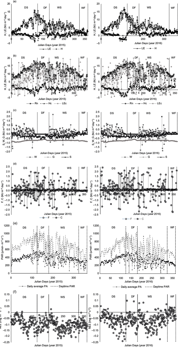
Fig. 2 Temporal variation of: (a) surface sensible heat flux (H) and surface latent heat flux (LE); (b) sensible heat flux at canopy height (Hc), latent heat flux at canopy height (LEc), and net radiation (Rn); (c) soil heat flux (G), soil heat storage (S), and water heat storage (W); (d) photosynthetic energy flux (F) and canopy heat storage (C); (e) photosynthetically active radiation (PAR); (f) net ecosystem exchange of carbon dioxide (NEE) during the dry season (DS), dry fallow (DF), wet season (WS) and wet fallow (WF) of 2015 and 2016
Table I Summary of components of energy balance (mean) and Bowen ratios for a lowland paddy
| Mean half-hourly value | DS | DF | WS | WF | ||||
| 2015 | 2016 | 2015 | 2016 | 2015 | 2016 | 2015 | 2016 | |
| Rsd | 18.02 (146%) | 17.23 (144%) | 18.09 (128%) | 17.80 (131%) | 14.98 (129%) | 15.27 (143%) | 12.19 (154%) | 14.53 (157%) |
| Rsu | 2.07 (17%) | 2.17 (18%) | 2.25 (16%) | 2.46 (18%) | 1.60 (14%) | 1.63 (15%) | 1.51 (19%) | 2.07 (22%) |
| Rld | -4.85 (-39%) | -4.49 (-38%) | -3.07 (-22%) | -3.16 (-23%) | -2.73 (-23%) | -2.76 (-26%) | -3.63 (-46%) | -4.41 (-48%) |
| Rlu | -0.41 (-3%) | -0.63 (-5%) | -0.49 (-3%) | -0.57 (-4%) | -0.24 (-2%) | -0.26 (-2%) | -0.24 (-3%) | -0.52 (-6%) |
| C | 0.03 (0.3%) | 0.21 (1.8%) | 0.31 (2%) | 0.52 (4%) | 0.14 (1%) | 0.69 (6%) | -0.34 (-4%) | 0.83 (9%) |
| G | -0.78 (-6%) | -0.80 (-7%) | -0.65 (-5%) | -0.71 (-5%) | -0.71 (-6%) | -0.77 (-7%) | -0.78 (-10%) | -0.87 (-9%) |
| S | -0.17 (-1%) | -0.18 (-1%) | -0.29 (-2%) | -0.23 (-2%) | -0.17 (-1%) | -0.11 (-1%) | 0.16 (2%) | 0.13 (1%) |
| W | 0.15 (1.2%) | 0.17 (1.4%) | 0.00 (0%) | 0.00 (0%) | 0.05 (0.5%) | 0.004 (0.04%) | 0.00 (0%) | 0.00 (0%) |
| F | 0.06 (0.5%) | 0.07 (0.6%) | 0.05 (0.4%) | 0.09 (0.6%) | 0.06 (0.5%) | 0.09 (0.9%) | 0.01 (0.1%) | 0.08 (0.9%) |
| Hc | 0.53 (4%) | -0.51 (-4%) | 1.41 (10%) | 2.12 (16%) | 0.86 (7%) | -0.32 (-3%) | 1.59 (20%) | 2.16 (23%) |
| LEc | 6.84 (55%) | 7.66 (64%) | 7.98 (56%) | 7.34 (54%) | 5.49 (47%) | 6.66 (63%) | 9.11 (115%) | 3.65 (39%) |
| Bc | 0.08 | 0.07 | 0.18 | 0.29 | 0.16 | 0.05 | 0.17 | 0.59 |
| H | 0.56 (5%) | 0.12 (1%) | 1.50 (11%) | 2.69 (20%) | 0.88 (8%) | 1.12 (11%) | 1.54 (19%) | 2.17 (23%) |
| LE | 6.82 (55%) | 7.90 (66%) | 8.50 (60%) | 7.96 (58%) | 5.30 (45%) | 5.09 (48%) | 2.53 (32%) | 2.58 (23%) |
| B | 0.27 | 0.15 | 0.21 | 0.38 | 0.23 | 0.25 | 0.64 | 0.89 |
| LE + H | 7.38 (60%) | 8.03 (67%) | 10.00 (71%) | 10.65 (78%) | 6.17 (53%) | 6.21 (58%) | 4.07 (51%) | 4.75 (51%) |
| V | 12.35 (100%) | 11.93 (100%) | 14.16 (100%) | 13.62 (100%) | 11.65 (100%) | 10.64 (100%) | 7.91 (100%) | 9.23 (100%) |
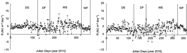
| R | 4.97 (40%) | 3.90 (33%) | 4.16 (29%) | 2.97 (22%) | 5.48 (47%) | 4.43 (42%) | 3.84 (49%) | 4.49 (49%) |
| Rn | 11.50 (93%) | 11.20 (94%) | 13.27 (94%) | 12.77 (94%) | 10.89 (93%) | 9.86 (93%) | 7.30 (92%) | 8.58 (93%) |
All the parameters shown in the table are average values of half hourly fluxes (MJ m-2 day-1), except for B and Bc, which are ratio of two energy fluxes. The value within the parenthesis express the percent of that component over the available heat flux.
Rsd: shortwave downwelling radiation; Rsu: shortwave upwelling radiation; Rld: longwave downwelling radiation; Rlu: longwave upwelling radiation; C: canopy heat storage; G: soil heat flux; S: soil heat storage; W: water heat storage; F: photosynthetic energy flux; Hc: sensible heat flux at canopy height; LEc: latent heat flux at canopy height; Bc: Bowen ratio at canopy height; H: surface sensible heat flux; LE: surface latent heat flux; B: Bowen ratio at surface; LE + H: turbulent heat flux; V: available heat flux; Rn: net radiation; DS: dry season; DF: dry fallow; WS: wet season; WF: wet fallow.
The temporal variation of G, S and W were shown in Figure 2c. S was observed as 0.17 MJ m-2 day-1 during DS, -0.29 MJ m-2 day-1 during DF, -0.17 MJ m-2 day-1 during WS and 0.16 MJ m-2 day-1 during WF in 2015. These values were 22.0, 44.1, 24.1, and 20.6% of the magnitude of G in that year. In 2016, S accounted for 22.4, 32.1, 13.9, and 15.4% of the magnitude of G. Water heat storage was recorded in cropping seasons only. The average energy stored in standing water (W) was three times higher in DS than in WS in 2015, while this value was much higher (42.5 times) in 2016. G was observed as -0.78 MJ m-2 day-1, -0.65 MJ m-2 day-1, -0.71 MJ m-2 day-1, and -0.78 MJ m-2 day-1 during DS, DF, WS and WF, respectively in 2015. This comprised 5-10% of the available energy (Table I). The value of G was slightly higher in 2016 with respect to all cropping seasons and fallows. The temporal variation of F ranged from 0.010 to 0.060 MJ m-2 day-1 in 2015 and 0.070 to 0.090 MJ m-2 day-1 in 2016 (Fig. 2d). The average highest F was noted in WS, while the lowest in WF. C was 0.3-9.0% of the available heat flux and DS showed less mean C than the DS (Fig. 2d).
The daily average PAR and daytime PAR from 6:00 to 18:00 local time (LT) (Fig. 2e) varied from 245.47-416.91 and 471.14-799.38 μmol m-2 s-1, respectively, in 2015, while in 2016 it was in the range of 20.6-550.3 and 39.6-1054.3 μmol m-2 s-1, respectively. The daily average PAR and daytime PAR had a higher value in DS and DF compared to the winter season in both years. The mean NEE ranged from -0.242 to 0.098 mg m-2 s-1 during the monitoring period including both crop seasons and the fallow period (Fig. 2f). The mean NEE during DS, DF, WS and WF were -0.070 mg, -0.065, -0.073, and -0.012 mg m-2 s-1, respectively, in 2015, and -0.086, -0.104, -0.110, and -0.099 mg m-2 s-1, respectively, in 2016. The magnitude of NEE was higher in 2016 compared to 2015.
3.3 Diurnal variation in behavior of energy fluxes
Rn reached its maximum at 11:30-12:00 LT during WS, 12:00 LT during WF, 12:30 LT during DS, and 11:00-13:00 LT during DF (Fig. 3a) during the study period. The time for the peak value of Rn varied in the second year for DF and WF. The magnitude of H reached its maximum at 12:00 LT for DS, 11:00-11:30 LT for DF, 12:00 LT for WS and 12:30 LT for WF. The average value of H was much higher in the fallow periods (DF and WF) than in the cropping seasons (DS and WS) during both years (Fig. 3b). The peak value of LE and G was reached at 12:30-13:30 LT and 9:00 -10:00 LT, respectively, in both years (Fig. 3c, d). The average seasonal G remained negative throughout the study period. The highest PAR was recorded at 12:00-12:30 LT for DS and DF, while at 11:30 LT for WS and WF in both years (Fig. 3e). The NEE remained negative during the sunshine period and the peak value was recorded at 11:30 -12:30 LT during both years (Fig. 3f).
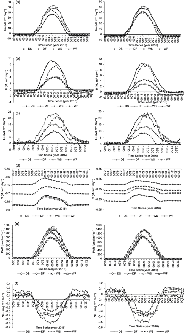
Fig. 3 Diurnal variation of (a) net radiation (Rn), (b) surface sensible heat flux (H), (c) surface latent heat flux (LE), (d) soil heat flux (G), (e) photosynthetically active radiation (PAR), and (f) net ecosystem exchange of carbon dioxide (NEE) during dry season (DS), dry fallow (DF), wet season (WS), and wet fallow (WF) of 2015 and 2016
3.4 Energy balance components
The key components of the EB were Rn, G, H and LE; however, when canopy was considered, S, W, F, and C were additional components for EB. G was recorded as -0.78, -0.65, -0.71, and -0.78 MJ m-2 day-1 for DS, DF, WS, and WF, respectively, in 2015 (Table I). The average values of G in DS, DF, WS and WF in 2016 were a little higher than in 2015. The value of F ranged from 0.1-0.6 MJ m-2 day-1 in 2015 to 0.07-0.09 MJ m-2 day-1 in 2016. The maximum average Hc and LEc were observed during WF (20-23% and 68-115% of the available energy, respectively) in 2015. Bowen ratio at canopy height (Bc) ranged from 0.08 to 0.18, while Bowen ratio at land surface (B) ranged from 0.21 to 0.64 in 2015 (Table I). The ranges of B and Bc were much wider in 2016. H was found to be higher in the fallow period than in the cropping season. The highest and lowest values of LE were registered in DF (58-60% of the available energy) and WF (28-32% of the available energy), respectively, during the period of study. The highest values of V and Rn were recorded in DF in both years, while R in WS during 2015 and WF during 2016.
3.5 Energy balance closure
Three ways were used to determine EBC, viz. OLS, EBR and RHF. In OLS, the coefficient of determination (R2) ranged from 0.66 to 0.85 for DS, 0.63 to 0.83 for DF, 0.38 to 0.49 for WS, and 0.67 to 0.80 for WF during 2015; and from 0.19 to 0.79 for DS, 0.20 to 0.74 for DF, 0.20 to 0.74 for WS, and 0.19 to 0.56 for WF during 2016 (Fig. 4). The value of R2 was higher than 60% in all seasons except in WS during both the years and WF in 2016. The slope was higher in DS (0.77-0.89) as compared to WS (0.38-0.47) in 2015 (Fig. 4). A similar trend was observed in 2016.
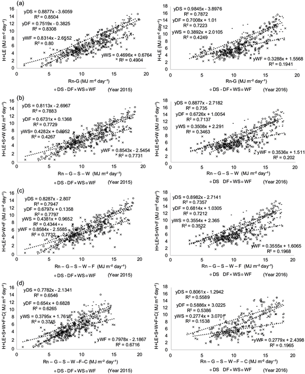
Fig. 4 Energy balance closure measurement by ordinary least square. (a) Rn - G vs H + LE. (b) Rn - G - S - W vs H + LE + S + W. (c) Rn - G - S - W - F vs H + LE + S + W + F. (d) Rn - G - S - W -F - C vs H + LE + S + W + F + C. All during dry season (DS), dry fallow (DF), wet season (WS) and wet fallow (WF) of 2015 and 2016.
Regarding EBR, the coefficients did not show much variation between the cropping seasons and fallows (Table II); however, the EBR value was lower in WS compared to DS and the fallow season during both years. The average value of R was 10.3-12.0% higher in WS as compared to DS during the study period; however, R was 8.3% higher in DF than in WF during 2015, while 24.8% higher in WF than in DF during 2016 (Fig. 5).
Table II Summary of energy balance closure using energy balance ratio
| Year | Seasons | I | II | III | IV | ||||||||
| LE + H | V | EBR I | LE + H + S + W | V - S - W | EBR II | LE + H + S + W + F | V - S - W - F | EBR III | LE + H + S +W + F + C | V - S - W - F - C | EBR IV | ||
| 2015 | DS | 922.9 | 1535.5 | 0.60 | 920.5 | 1537.9 | 0.60 | 927.7 | 1530.7 | 0.61 | 931.1 | 1527.3 | 0.61 |
| DF | 560.0 | 779.7 | 0.72 | 543.8 | 795.8 | 0.68 | 546.8 | 792.9 | 0.69 | 557.5 | 782.2 | 0.71 | |
| WS | 883.0 | 1658.1 | 0.53 | 866.3 | 1674.7 | 0.52 | 874.9 | 1666.2 | 0.53 | 884.7 | 1656.3 | 0.53 | |
| WF | 167.0 | 331.2 | 0.50 | 173.5 | 324.6 | 0.53 | 173.9 | 324.2 | 0.54 | 171.5 | 326.6 | 0.53 | |
| 2016 | DS | 1003.5 | 1499.3 | 0.67 | 1002.7 | 1500.1 | 0.67 | 1011.6 | 1491.2 | 0.68 | 1037.8 | 1465.0 | 0.71 |
| DF | 596.6 | 755.0 | 0.79 | 583.8 | 767.7 | 0.76 | 588.7 | 762.9 | 0.77 | 616.4 | 735.2 | 0.84 | |
| WS | 888.2 | 1520.5 | 0.58 | 873.5 | 1535.2 | 0.57 | 886.6 | 1522.2 | 0.58 | 984.3 | 1424.4 | 0.69 | |
| WF | 200.1 | 395.7 | 0.51 | 205.7 | 390.1 | 0.53 | 209.2 | 386.6 | 0.54 | 223.4 | 372.3 | 0.60 | |
All the parameters shown in the table are the average values of the half-hourly fluxes (MJ m-2 day-1), except for EBR I-IV, which are ratios.
LE + H: turbulent heat flux; V: available heat flux; S: soil heat storage; W: water heat storage; F: photosynthetic energy flux; C: canopy heat storage; EBR: energy balance ratio; DS: dry season; DF: dry fallow; WS: wet season; WF: wet fallow.
4. Discussion
4.1 Temperature, precipitation, and wind characteristics of the site
Mean daily temperature was higher in DF than other seasons. Rn had a closer relation with daily temperature. Since higher Rn was received during that period, daily temperature was higher. Clouds have a significant role in the uncertainty of the energy budget measurement, as does Rn by affecting shortwave and longwave radiations (Matus and L’Ecuyer, 2017). Specific humidity (q) is not directly obtained from eddy data, rather it is derived (Gao et al., 2003):
where RH is measured in EC and q sat is the saturated specific humidity (derived).
Again, q sat is derived from the following equation:
where p is the measured air pressure (kPa) and e sat is saturated vapor pressure (kPa), which is low due to higher occurrence of rainfall in WS, resulting in lower specific humidity in that season. However, there is uncertainty in the measurement of qa, since it is a derived term; likely as a result of this, the value of qa was found very close to zero. Maximum precipitation was received during WS, which coincides with the south-west monsoon period in India. Wind speed and wind direction varied with respect to different seasons. The monsoonal circulation is due to temperature differences between land and sea triggered by insolation (Huffman et al., 1997). During winter, less solar radiation is intercepted at the northern hemisphere, which results in rapid cooling of the earth surface followed by an increase in pressure in the atmosphere. On the contrary, during summer, warming of the northern hemisphere controls the south-west monsoon (Wolfson, 2012). Due to such variation in air temperature and pressure, wind blows in a variable direction with varying speed in different seasons.
4.2 Variation of energy fluxes between cropping seasons and fallows
Hc was lower than LEc throughout the year, which is due to standing water in the rice field throughout the cropping seasons. The non-limiting water supply increased concurrently evapotranspiration in the rice canopy and evaporation from the soil surface. The combined effect increased LEc over Hc in all seasons across years. During daytime, Rn was the principal contributor of energy flux to the surface, whereas LE was the main receiver from the surface; during nighttime, G and S were the chief energy contributors, and Rn as well as LE were the main receivers (Swain et al., 2018a). The value of G was slightly higher in 2016 with respect to all cropping seasons and fallows, which may be due to a higher amount of cloud free days during 2016 (Fig. 1c). The average energy stored in soil (S) and standing water (W) was higher in DS than in WS, which may be due to higher insolation during DS (Roxy et al., 2014). The magnitude of F was much lower compared to the available heat flux. F (biochemical energy stored by photosynthesis) is generally within 1-2% of the available heat flux (Liu et al., 2017), which can be reconfirmed in this experiment. A significant value of F was recorded in DF during 2015, as well as in DF and WF during 2016 due to the presence of ratoons of rice (new tillers sprouted from the stubble) and weed in the field promoted by occasional pre and post monsoon rainfall. Interestingly, C is often neglected in energy balance studies (Gao et al., 2003). C was higher in WS than in DS, which may be due to higher biomass and longer duration of the variety in the WS. In this study, F and C have been considered in the correction of energy balance deficits. The daily average PAR was much higher in DS and DF as compared to WS and WF. This is again due to overcast or cloudy conditions during the monsoon season (June to September), which leads less insolation during the wet season (Alberto et al., 2009). The NEE of lowland rice was mainly controlled by numerous environmental variables and ecosystem parameters such as LE, heat stress, canopy irradiance, stomatal resistance evaporative demand, leaf area index, vapor pressure deficit, stages of rice growth, biomass, etc. (Nair et al., 2011). More negative NEE was observed during daytime due to the increase in photosynthetic CO2 assimilation (increase in GPP) as Rn increases (Alberto et al., 2009). Higher negative NEE with the increase in PAR and Rn was also observed in this study (Swain et al., 2018b). Assimilation during the fallow seasons (-0.065 and -0.012 mg m-2 s-1 in DF and WF, respectively) may be attributed to the ratoons of rice and weeds present in the site (Miyata et al., 2000). A high B was observed in WF compared to DF (Table I). Actually, pre-monsoon shower is received in this region during DF. However, during WF no occasional rainfall is received (Fig. 1c). Therefore, H is dominated in WF compared to DF which is reflected in higher B in WF.
4.3 Diurnal variation in the behavior of energy fluxes
Diurnal variations of monthly and seasonal averaged EB components varied in a unimodal shape. Generally, the values of Rn, G, LE and H gradually decreased with decreasing insolation from the sun. As compared with H and G, diurnal variation amplitude of LE was much greater. The dominant component of Rn in the rice paddy was LE, and the magnitude of G and H was comparatively low during the crop season. H was consistently near zero or negative before sunrise and after sunset, primarily because insolation was absent and there was very little turbulence during those hours. Positive upward H during daytime was primarily due to insolation and increased turbulence (Montazar et al., 2016). As compared to Rn, the daily dynamics of G showed a few hours delay in the early morning and started to change after the sun rise. This could be due to changes in the rice crop height (1.2 m), which induced a delay in soil surface warming (Gao et al., 2009; Roxy et al., 2014). The diurnal variation in G in different season, including the fallows, may be caused by many reasons such as rainfall events, soil moisture conditions, net radiation, skin temperature, vegetation, etc. PAR also followed the same trend as Rn (Tsai et al., 2007). On diurnal basis, the rice crop behaved as net CO2 sink except for the night hours. Diurnal variation in NEE amplified with the progress of day, attained maximum around noon and then decreased gradually until evening (Pakoktom et al., 2009; Swain et al., 2018b). Besides radiation and the time of day, several other factors influenced NEE, like air temperature, soil temperature, vapor pressure deficit, PAR, water vapor flux and soil moisture content (Bhattacharyya et al., 2013; Chatterjee et al., 2019b).
4.4 Energy balance closure
The surface energy budget closure (EBR I) was measured by taking the (H + LE):(Rn - G) ratio, and consecutive terms (S, W, C, F) were taken into account in different combinations to calculate EBR II-IV (Table II) (Tsai et al., 2007). Ideally, EBR must be 1 when the surface energy balance is perfectly closed (Gu et al., 1999). This study shows that the highest mean value of EBR I among the four seasons was 0.72 in DF during 2015. This implies that only 72% of the available energy (V) was balanced by cumulative turbulent heat flux (H + LE) during this period. This value falls further in DS (0.60), WS (0.53), and WF (0.50) in 2015. A similar trend was observed in 2016. Higher energy imbalance in WS and WF mainly happened after the rainfall events. DS and DF were almost free from rainfall, except for a few overcast days (Fig. 1c). Hence, the energy components showed better balance during the rain-free days. When applying the correction to H and LE by adding the storage term, a new and improved EBC can be obtained (Moderow et al., 2009). These new closures (EBR II-IV) did not have an important impact on energy balance in DS since the values were 0.58, 0.59, and 0.60, which was too close to EBR I (2015). The same phenomenon applies for the rest of the seasons (DF, WS and WF). EBR values (I-IV) in 2016 were a little higher than in 2015, showing better energy balance in this last year.
Linear regression coefficients from the OLS relationship showed a better coefficient of determination (R2) in DS, DF and WF compared to WS. This may be due to higher precipitation and overcast days in WS. The closure is achieved in OLS when the magnitudes of intercept and slope are zero and 1, respectively (Liu et al., 2017). In this study, the slope was higher in DS, DF, and WF compared to WS during both years (Fig. 4). This indicates that the energy balance was better in DS, DF, and WF compared to WS. Unlike Tsai et al. (2007), who observed an increase in the slope and decrease in the coefficient of determination (R2), we observed a decrease both in slope and R2 with the incorporation of the storage component in the closure. Lowering of slope may be due to decrease in cumulative turbulent flux and increase in available heat flux when the storage term is added.
A comparison between all seasons showed that average RHF was increasing positively from DS to WF (Fig. 5) and it should be equal to zero when the surface energy budget is perfectly closed. Since the average value of RHF is more than zero in all seasons across years, the available heat flux was greater than the cumulative turbulent flux (Liu et al., 2017). This imbalance is much more in WS and WF. Among the three ways of EBC measurements, it was observed that average values of RHF can clearly distinguish the various cropping seasons and fallows in the study of energy balance closure in a lowland paddy.
Effective closure of the surface energy balance provides a high level of confidence on the flux observation method. Imperfect closure denotes measuring errors of the eddy covariance system or failure to include the heat storage measurement. However, recent studies show that imperfect EBC is a scale problem (Masseroni et al., 2014). Assessment of the EBC is accepted as an important procedure for evaluating data quality (Aubinet et al., 2000). The interaction of measurement errors of raw CO2 fluxes is directly related to incomplete EBC (Liu et al., 2006). The magnitude of CO2 fluxes using an open-path infrared gas analyzer is largely overestimated, thus the WPL algorithm associated with this flux is underestimated (Anthoni et al., 2002).
Cloudiness impacts shortwave and longwave radiations, which ultimately impact the net radiation of the rice cropping system. Again, clouds heat the tropical atmosphere by increasing the greenhouse effect, hence cloudiness exerts some uncertainty in the measurement of EBC.
Changes in water depth during WS contribute to difficulties in closing the energy budget. Rainfall brings fresh water into the system, which results in advection of energy into the system. Moreover, maintaining the standard depth of water in WS is also difficult after a rainfall event. More uncertainty was involved in the measurement of EBC in WS.
5. Conclusions
There are several factors that prevent the achievement of a perfect closure, such as landscape heterogeneity, errors in flux observations, averaging periods and coordinate systems, horizontal advection, instrument bias, or a combination of several issues (Reed et al., 2018). The following conclusions can be drawn from this study:
Unlike other arable crops, in rice paddies the flooding of land and the maintenance of standing water over a land surface largely alter the typical energy balance measurements. As heat is stored in the standing water, among all the energy components, in a lowland rice paddy LE is the dominant element and controls the energy budget. Similarly, LEc dominates over Hc.
In a lowland irrigated rice paddy, the RHF for estimating EBC is the most appropriate way, since it can clearly distinguish between different seasons and fallows.
Estimation of the heat storage term can improve EBC.
However, measurement errors or storage terms are not always useful for a perfectly closed energy balance. EBR did not show much variation after the inclusion of storage terms (water, soil, photosynthesis, canopy) to EBR I (H + LE vs Rn - G). Hence, energy exchange processes based on a point measurement over a small landscape may lead to an imperfect energy balance closure. This situation will probably be improved when a comparatively larger area is considered. EBC is probably a scale problem which may have an important role in the measurement of turbulent fluxes.

