1. Introduction

Mean air temperature (from now on mean temperature), has a high impact on electric power generation, which is one of the most important economic activities in Argentina, as it affects gas consumption directly (^{Gil et al., 2005}). Considering this impact, it is relevant to analyze the interannual variability of atmospheric temperature, for which it is necessary to know the influence of global and regional factors. It is known that there is a strong relationship between El Niño Southern Oscillation (ENSO) phenomenon and mean temperature in Argentina, for instance, positive temperature anomalies in southern Patagonia and negative anomalies in subtropical latitudes are observed during the preceding winter of a positive ENSO phase. Also, these positive anomalies extend north of Buenos Aires Province during the preceding spring of a positive phase. Opposite patterns are observed during winter and spring of the same year of a warm ENSO event (^{Kiladis and Díaz, 1989}).

^{Rusticucci et al. (2003)} found that seasonal occurrence of cold and warm events in Argentina, defined by daily extreme temperatures, are related to the cooling and warming of coastal waters of the South Atlantic and South Pacific oceans. According to their study, there is a fair degree of predictability of these events based on the Atlantic and Pacific sea surface temperature (SST), especially in winter, with higher correlations with the Atlantic than with the Pacific Ocean, as the Andes represent a significant orographic barrier. ^{Barrucand et al. (2008)} observed the most significant association with the Atlantic SST of coastal zones in the frequency of warm events in the central-east and northeast of Argentina. The present work aimed to find the relationship between the SST of the Atlantic and Pacific coastal oceans, and the mean inland temperatures in Argentina.

This paper is organized as follows: section 2 details the data employed in this study, section 3 determines the variability patterns of SST, section 4 analyzes the relationship between these patterns and mean temperature, and section 5 presents the conclusions.

2. Data

Monthly SST data from the ERA-Interim reanalysis (^{Dee et al., 2011}) of the European Centre of Medium-Range Weather Forecast, with 0.75º resolution (downloaded from http://www.ecmwf.int/en/forecasts/datasets) were used to obtain seasonal averages for the period 1980-2015. Seasons were defined as DJF (summer), MAM (autumn), JJA (winter) and SON (spring). These averages were performed over a study region delimited by 20-60º S and 30-90º W, to analyze the interannual variability of the coastal SST values, and to detect its contribution to mean seasonal temperature in Argentina.

The National Meteorological Service of Argentina provided monthly mean temperature data from 67 weather stations (Fig. 1). Seasonal averages from DJF 1980 until DJF 2015 were obtained from these stations (observations were not available beyond March 2015).

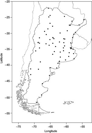
Fig. 1 Study area. Black dots show the weather stations locations. The longitudinal extent of this study is broader (90 to 30º W). 

Composites of 850 hPa wind anomaly from the NCEP/NCAR reanalysis (^{Kalnay et al., 1996}) provided by the NOAA-ESRL Physical Sciences Division (from their webiste at http://www.esrl.noaa.gov/psd/) were used. For these data, the employed climatology period was from 1981 to 2010.

3. Variability patterns of seasonal SST

Interannual variability of summer and winter SST was studied through principal component analysis (PCA) derived patterns on T-mode (^{Preisendorfer, 1988}). In this mode, the variables are the spatial fields defined by m grid points, at each of the n times. In this work spatial fields of seasonal (summer or winter) SST anomalies were considered.

The study region was delimited by 30-90º W and 20-60º S, with a 0.75º spacing between grid points, comprising a total number of 4455 m points. The analyzed period from 1980-2015 (i.e., n = 36 years) comprises 36 input variables. If the standardized (by the mean and standard deviation of each column) data matrix X _s is the input matrix of PCA, the three output arrays are (^{Compagnucci and Salles, 1997}):

The new variables, now called principal components (PCs), are the columns of Z _s and they are the spatial patterns in the T-mode, while F columns or PC component loadings (PCLs) are the time series. PCLs are conformed by correlation coefficients between the original variables and the corresponding principal component. F has two interesting properties: the sum of the squared loadings of each component equals its respective eigenvalue, and similarly, the sum of the squared entries of each variable equals its respective variance (^{Carroll et al., 1997}), which is equal to 1 for standardized variables. This means that the sum of all the eigenvalues equals the total variance and so the i-th PC accounts for λ _i /∑ ^r _j=1 λ _j of the total variance.

In this work, the PCA technique was applied through singular value decomposition (SVD) from which the same arrays D, F and Z _s can be obtained (^{Green, 1978}; ^{Mestas-Núñez, 2000}; ^{Compagnucci et al., 2001}; ^{Compagnucci and Richman, 2008}). Spatial patterns and time series given by PC and PCL, respectively, represent interannual variability patterns of summer (section 3.1) and winter (section 3.2) SST.

3.1 Summer patterns

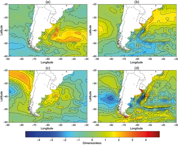
A subjective (non-statistically inferred) truncation criteria was applied to select the optimum number of PCs. To do so, the PCs must explain an important proportion of total variance and also show spatial patterns with physical meaning. The truncation cutoff for the principal components was taken following a scree test. This test consists of identifying a point at the eigenvalue spectrum plot (λ _i vs. i), which separates a steeply sloping portion to the left, and a more shallowly sloping portion to the right. The principal component number at which the separation occurs is taken as the truncation cutoff. For the summer patterns, this cutoff was at seven PCs. Similarly, according to the Kaiser criterion (PCs whose eigenvalue is greater than 1), eight PCs should have been retained (^{Wilks, 2006}). The explained variance for the first eight PCs is shown in Table I, accounting for more than 80% of the total variance altogether and 60% if only the first four are considered. Spatial patterns of the SST anomaly given by the first four PCs are shown in Figure 2 and described below:

• PC 1 showed a warm center over the Atlantic and a cold center over the Pacific off the southern Patagonian coast (Fig. 2a).

• PC 2 consisted of warmer temperature anomalies in the Atlantic Ocean which extended from southern Brazil to the coastal waters of Uruguay and Buenos Aires, south of which colder temperatures were observed. Over the Pacific Ocean SST anomalies were warmer than those found on PC1, but less warm than the Atlantic anomalies (Fig. 2b).

• PC 3 showed warmer anomalies over the Pacific Ocean, off the north coast of Chile, and over the Atlantic, off the coast of Buenos Aires and Patagonia. Further out from the coast, colder anomalies were seen off the coast of Chile and Argentina (Fig. 2c).

• PC 4 was characterized by a cold center over the Pacific Ocean, off the southern Chilean coast. Over the Atlantic cooling off the Patagonian coast and warming off the Buenos Aires coast was observed. Further east, the pattern was unclear (Fig. 2d).

Table I Percentage of explained variance for summer (DJF). 

	PC 1	PC 2	PC 3	PC 4	PC 5	PC 6	PC 7	PC 8
Explained variance (%)	22.98	19.77	11.11	7.75	6.68	6.31	3.43	3.26
Cumulative explained variance (%)	22.98	42.75	53.86	61.61	68.29	74.6	78.03	81.29

Fig. 2 Summer (DJF) principal components: (a) PC 1, (b) PC 2, (c) PC 3 and(d) PC 4. 

As the pattern represented by PC 4 had an important spatial variability, an analysis was made only for the first three PCs, which accounted for 23%, 19.8% and 11.1% of the total variance, respectively (53.9% in total). The time series represented by the first three PCLs are displayed in Figure 3. Each of them shows the correlation value between the corresponding PC and the summer SST anomaly field of each year of the considered period. The most highly correlated years of each PC were defined as follows: the years whose correlation value was greater than a cutoff value, given by the mean of the absolute value of all the correlations plus a standard deviation (see Table II).

Fig. 3 Summer (DJF) PC loadings: (a) PCL 1, (b) PCL 2 and (c) PCL 3. 

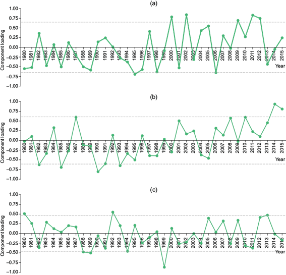
Table II Best correlated years between summer SST anomalies and the first three PCs. Cutoff correlation values are shown. 

	PC 1	PC 2	PC 3
Cutoff value	0.65	0.61	0.46
Positive correlation	2000, 2002, 2009, 2011, 2012	2014, 2015	1980, 1992, 2013
Negative correlation	1995, 2006	1982, 1985, 1990, 1993	1988, 1989, 1999

3.2 Winter patterns

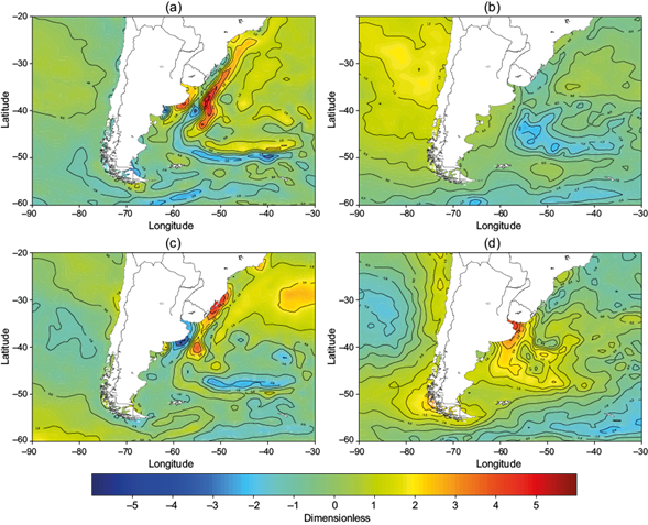
Based on the scree test, the number of winter PCs that should have been retained was seven. Eigenvalues greater than 1 corresponded only to the first eight PCs. The explained variance by the first eight PCs is shown in Table III, which accounted for 75% of the total variance, and almost 60% only considering the first four components. The spatial patterns of SST anomalies given by the first four PCs are shown in Figure 4, and described below.

Table III As in Table I, but for winter (JJA). 

	PC 1	PC 2	PC 3	PC 4	PC 5	PC 6	PC 7	PC 8
Explained variance (%)	28.90	12.92	9.59	6.58	6.20	4.75	3.28	3.08
Cumulative explained variance (%)	28.90	41.82	51.41	57.99	64.19	68.94	72.22	75.30

• PC 1 showed maximum variability over the Atlantic Ocean, with the main warm center extending to the northeast, from Patagonia to southern Brazil. Off the coast of Buenos Aires, a warm center in the north and a cold one in the south were recorded. In between these centers, a cold center was observed reaching Patagonia, which extended eastwards. South of 50° S, cooling was seen over the Atlantic Ocean. In addition, the coastal waters of the Pacific Ocean exhibited slightly cold anomalies (Fig. 4a).

• PC 2 was characterized by warming over the Pacific Ocean with a maximum to the north, and a cold center over the Atlantic Ocean some distance away from the northern Patagonia coast. There were other cold centers over the ocean, south of Patagonia (Fig. 4b).

• PC 3 showed a cold center off the coast of Buenos Aires, and a warm center east of it, which reached southern Brazil. East of these main centers, the ocean was warm to the north and mostly cold to the south. The coastal Pacific presented weak anomalies (Fig. 4c).

• PC 4 exhibited a cold center over the subtropical Pacific and slight warming along the length of the nearshore coastal waters, while the Atlantic showed positive anomalies over its center, especially off the Buenos Aires coast. Cooling to the north and the south of this area was recorded, which was stronger in the south (Fig. 4d).

Fig. 4 As in Figure 2, but for winter (JJA). 

The analysis of the next sections includes the four first PCs, as all of them showed clear spatial patterns and accounted for 58% of the total variance (28.9% by PC 1, 12.9 % by PC 2, 9.6% by PC 3, and 6.6% by PC 4). The time series represented by the first four PCLs are displayed in Figure 5. Cutoff correlation value and most highly correlated years were chosen using the same criterion as for summer PCs (Table IV).

Fig. 5 As in Figure 3, but for winter (JJA) and (d) PCL 4. 

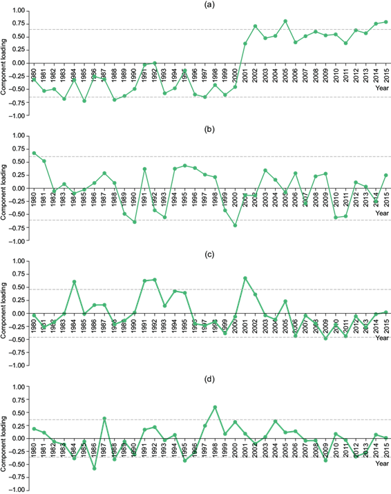
Table IV As in Table II, but for winter (JJA). 

	PC 1	PC 2	PC 3	PC 4
Cutoff value	0.69	0.49	0.43	0.36
Positive correlation	2002, 2005, 2014, 2015	1980, 1981	1984, 1991, 1992, 2001	1987, 1998
Negative correlation	1985, 1988	1989, 1990, 1993, 2000, 2010, 2011	2006, 2009, 2011	1984, 1986, 1988, 1995, 2009

4. Relationships between variability patterns of SST and seasonal mean temperature

Linear correlations between PCLs from interannual variability modes of seasonal (summer and winter) SST and simultaneous series of mean temperatures were calculated, to find a relationship between both variables. To evaluate the predictability of seasonal mean temperature, lagged-by-one-season correlations were also performed (i.e., summer PCLs with autumn temperature and winter PCLs with spring temperature).

The significance of Pearson correlation coefficient was tested by a two-tailed t-test with a confidence level of 95%. The test statistic used was T=Rn-21-R2 and n -2 the degrees of freedom (^{Devore, 2011}). The degree of freedom for correlations that involved summer series was 34, whereas for autumn, winter and spring it was 33. Therefore, in all these cases, a correlation coefficient of 0.34 was required for a significant linear relationship with a confidence level of 95%. Correlation distributions were performed by interpolating correlation values using a Cubic Spline method. Obtained results are discussed in section 4.1 for SST variability patterns of both summer (section 4.1.1) and winter (section 4.1.2). In section 4.2 some processes which would connect variability patterns of SST and simultaneous seasonal mean temperature of Argentina, are analyzed.

4.1. Variability patterns of SST and mean temperature

4.1.1. Summer

The first variability pattern of summer SST did not show association with simultaneous mean temperature in Argentina, since PCL 1 was significantly correlated with mean temperature series only at an isolated meteorological station in Patagonia (Comodoro Rivadavia Aero: 87860). The second pattern (the second pattern but with opposite sign anomalies) showed association with simultaneous warm (cold) anomalies over a large area of northern and west-central Argentina (Fig.6a). Correlation values between PCL2 and the simultaneous mean temperature series were significant in almost half of all meteorological stations. This suggests that warm (cold) anomalies over the coastal Atlantic, north of Buenos Aires, and cold (warm) to the south, and the warm (cold) anomalies over the Pacific, at the center of the study region, contribute to warmer (colder) than normal summers at northern and west-central Argentina. The third pattern (the third pattern but with opposite sign anomalies) was related to positive (negative) anomalies of simultaneous mean temperature just over a small area of northeastern Argentina (Misiones province). Lagged correlations (not shown) showed a poor relationship between summer SST variability modes and autumn mean temperature.

Fig. 6 Distribution of the Pearson correlation coefficient between PCLs and mean temperature series: (a) DJF PCL 2 and simultaneous series, (b) JJA PCL 1 and simultaneous series, (c) JJA PCL 1 and (d) lagged series and JJA PCL 3 and simultaneous series. Blue and red colors denote negative and positive correlations, respectively, with a significant confidence level of 95%. 

4.1.2 Winter

The first variability pattern of winter SST (the first pattern but with opposite sign anomalies) showed association with simultaneous warm (cold) anomalies in the north and center-west of Argentina (Fig. 6b). This indicates that an anomalously warm (cold) Atlantic Ocean close to the north of Buenos Aires and cold (warm) to the south, may be accompanied by a warmer (colder) winter than normal in northern and west-central Argentina. This relationship is maintained until the following spring according to the lagged correlation and, in this case, the area with significant values was larger than the simultaneous one (Fig. 6c). This could mean that there is a good degree of predictability of mean temperature from the first variability pattern of winter SST.

The correlation distribution corresponding to PCL 2 and the simultaneous mean temperature series had no significant areas, so the second variability pattern of winter SST could not be related to winter mean temperature. The correlation value resulted significant only at an isolated meteorological station in northeastern Argentina (Iguazú Aero: 87097).

Besides the first pattern, the third pattern (the third pattern but with opposite sign anomalies) also showed a good relation to the simultaneous mean temperature in Argentina. It showed association with cold (warm) simultaneous mean temperature anomalies in most of Patagonia and the south of Buenos Aires province (Fig. 6d). This suggests that a mostly cold (warm) southern Atlantic Ocean, with a pronounced cooling (warming) near Buenos Aires coast and warm (cold) anomalies near the southern coast of Brazil, which extend to south, east of Río de la Plata, promote anomalously cold (warm) winters in Argentinian Patagonia.

PCL 4 was positively correlated with simultaneous mean temperature series of all the meteorological stations considered. Nonetheless, these correlations resulted significant just over the east of Buenos Aires province, and only in this area, the fourth variability pattern of winter SST (the fourth pattern but with opposite sign anomalies) could be associated with positive (negative) anomalies of mean temperature.

Besides the first variability mode, the other winter variability modes did not show an important relationship with spring mean temperature.

4.2 Hypotheses that may explain the relationship between variability patterns of SST and seasonal mean temperature

Additional analysis was conducted for those PCs whose associated PCLs showed the most important significant correlations with simultaneous seasonal mean temperature, to find processes which may lead to this relationship. Seasonal composites of the 850 hPa wind anomaly of the best correlated years (according to the criterion explained in section 3) were studied, taking separately those years which were positively correlated (hereafter “+ Years”) and those which were negatively correlated (hereafter “- Years”). Thus, in + Years the SST anomaly patterns were similar to the corresponding PC and in - Years the patterns were similar to the opposite to the one displayed (i.e., cold where it is warm, etc.).

Some hypotheses about the processes which may contribute to the explanation of the observed correlations are exposed below. It is necessary to take into consideration that composite fields were performed in general with a few cases, and also that not all the correlations of + Years and - Years with the corresponding PC were equally high.

Summer PC 2 (Fig. 2b) is associated with warm anomalies over north and center-west of Argentina, as it was described above. Both subtropical high and subpolar low were intensified, leading to more intense westerlies (Fig. 7a) in the case of + Years (2014, 2015), so it was less probable that frontal perturbations moved northward (^{Silvestri and Vera, 2003}; ^{Reboita et al., 2009}). In summer, less frontal precipitation is associated with higher temperatures. Besides, the Atlantic Ocean was probably anomalously warm in the north because of the similarity of +Years patterns to PC 2, so the north-northeastern flow which came from the anticyclone, increased the warming, especially in northern Argentina where the northern flow (low-level jet) prevails in summer. Consequently, a relationship between this pattern and higher temperatures in northern Argentina is logical. The opposite was observed in - Years (1982, 1985, 1990, 1993), when wind anomalies showed both weaker-than-normal subtropical high and subpolar low (Fig. 7b).

Fig. 7 Summer (DJF) composite of (a) 850 hPa wind anomaly (m/s) of the + Years and (b) - Years defined for the summer PC 2. 

Winter PC 1 (Fig. 4a) showed association with warm anomalies in northern and west-central Argentina. Air advection from the north prevailed over northern and, especially, northeastern Argentina (Fig. 8a) in the + Years (2002, 2005, 2014, 2015), leading to higher temperatures there. This effect would have been enhanced if the Atlantic Ocean was warm in the area where the anticyclone enters the continent, which is probable since the + Years patterns were similar to PC 1. In contrast, in the - Years (1985, 1988) wind was anomalously easterly (Fig. 8b) and came from a portion of the Atlantic that was probably cooler than normal.

Fig. 8 As in Figure 7, but for winter (JJA) and PC 1. 

Winter PC 3 (Fig. 4c) is related to cold anomalies over most of Patagonia and the south of Buenos Aires province. Easterly wind anomalies were observed in southern Argentina (Fig. 9a), reflecting an important weakening of the westerlies in + Years (1984, 1991, 1992, 2001). Because of + Years patterns similarity to PC 3, this meant enhanced possibilities of cold advection from a cooler-than-normal Atlantic Ocean towards Patagonia and, therefore, of lower-than-normal temperatures there. On the other hand, there were very slight anomalies over the Atlantic Ocean close to Patagonia in the case of - Years (2006, 2009, 2011) composite (Fig. 9b). This effect does not seem to explain the important signal observed over Patagonia only by itself, as the SST anomalies over the nearby ocean were not so high. Probably, other factors enhanced this signal (for instance, weakened westerlies imply more fronts passing through and therefore higher cloud cover, associated with lower mean temperature).

Fig. 9 As in Figure 7, but for winter (JJA) and PC 3. 

5. Conclusions

Results showed a relationship between coastal oceans SST and mean temperature in Argentina. Particularly, warm (cold) anomalies over the nearby Atlantic, north of Buenos Aires and cold (warm) to the south, and the nearby Pacific anomalously warm (cold) at the center of the study region, are associated with warmer (colder) than normal summers at northern and west-central Argentina. Besides, an anomalously warm (cold) Atlantic Ocean close to the north of Buenos Aires and cold (warm) to the south contribute with warmer (colder) than normal winters in northern and west-central Argentina. This pattern also affects the following spring in the same way, but over a larger area. Also, a mostly cold (warm) southern Atlantic Ocean, with a pronounced cooling (warming) near Buenos Aires coast and warm (cold) anomalies near southern coast of Brazil which extend to south, east of Río de la Plata, are related to anomalously cold (warm) winters in Argentinian Patagonia.

Findings of this study suggested that there is a good degree of predictability of spring mean temperature from a winter SST pattern, which accounts for almost 29% of the total variance. In contrast, autumn mean temperature seems to have a poor relationship with SST summer patterns.