


 text new page (beta)
 English (pdf)
 Article in xml format
 Article references
 Send this article by e-mail
 Cited by SciELO
  Similars in
SciELO
Similars in
SciELO 
 Permalink
1. Introduction
Argentina is in southeastern South America, occupying a total area of 2 791 810 km2. Because of its extensive territory, there are areas with different climate features and rainfall can be linked to many different factors. Several authors have studied rainfall in this region according to different forcings, mainly the sea surface temperature (SST), which in turn shows a strong influence on the Atlantic Ocean and its circulation (Doyle and Barros, 2002; Barros et al., 2008; Barreiro, 2010). However, there are only a few works that address the study from the behavior of the semi-permanent South Atlantic High (AH).
Big oceans that cover the earth act as important reservoirs of heat and thus are essential to study climate forcings of rainfall. In particular, the Atlantic Ocean is an important factor that affects precipitation because SST and its variability can be associated with humidity availability and its advection towards southern South America. The Atlantic Ocean’s SST and the atmospheric circulation that the semi-permanent South AH establishes, both regulate the advection of humid air produced towards Argentina and, particularly during austral spring and summer, affect the intensity of the South American Monsoon that advects humid air from the Brazilian rainforest to northern Argentina.
According to Cabos et al. (2017), the prescription of the AH south of 20º S improves the simulation of the seasonal cycle over the tropical Atlantic, revealing the fundamental role of this anticyclone in shaping the climate over this region. Sun et al. (2017) analyzed the annual cycle of the South AH and its interannual variability in connection with regional and large-scale climate variability. They found that the AH has an annual cycle of two peaks in intensity and size, being farthest poleward and in the central region of the South Atlantic basin during austral summer and less intense and closest to the equator and the western side of the basin in winter. In addition to this, they found that AH is strongest and largest during the solstitial months. Garbarini (2016) found similar results, showing that the AH increases its intensity during winter with its highest intensity in July and August with values over 2000 gpm. From austral winter onwards, the AH is located north of 30º S until November when it starts shifting south. On the other hand, the AH moves to the east of its mean position during winter reaching the Greenwich parallel and starts its shift towards the American continent in October.
Di Luca et al. (2006) applied a T-mode principal component analysis to monthly mean sea surface pressure and determined three predominant patterns. The fist pattern represents the summer surface circulation with the South Atlantic and South Pacific Highs in their southernmost positions. The second and third modes represent the winter circulation with the South Atlantic and South Pacific in their northernmost position and a surface pattern that characterizes the frontal activity during that season, respectively. Moreover, some results show trends in the location, a southward shift of the South AH (Camilloni, 1999; Camilloni et al., 2005) and a displacement to the south of the regional atmospheric circulation over southeastern South America (Barros et al., 2000).
When studying potential drivers of seasonal trends of heat fluxes between the atmosphere and the South Atlantic Ocean, Leyba et al. (2018) found that there has been an expansion and intensification of the Semi-Permanent Subtropical Anticyclone during the second half of the period 1982-2015. In consequence, there has been an intensification of the gradient pressure, causing an increase in wind speed, which leads to an increase in SST and therefore an intensification of air-sea heat fluxes in the region.
In addition, many different authors have studied how Atlantic and Pacific SSTs are connected to positive and negative air temperature anomalies in different regions of Argentina (Rusticucci et al., 2003; Barrucand et al., 2008). Some have also found connections between rainfall anomalies and atmospheric circulation in different regions of South America (González et al., 2016; Barrucand et al., 2007; Grimm, 2011; Grimm and Ambrizzi, 2009, among others).
The aim of this work is to study the relation between SST anomalies in the South Atlantic Ocean and the semi-permanent South Atlantic High. This preliminary analysis will eventually help to determine the influence of these variables over seasonal precipitation anomalies in Argentina to create seasonal forecasts.
For this purpose, this paper is structured in four sections. Section 2 shows the datasets used for this study and the methodology employed for the subsequent analysis. Sections 3.1 and 3.2 describe the variability patterns of both variables, while 3.3 explores the connection between SST and geopotential height in the 1000 hPa level (HGT1000) using linear correlations. Finally, section 4 summarizes the conclusions.
2. Data and methodology
Seasonal SST and HGT1000 from the NCEP/NCAR reanalysis for the 1981-2016 period were used, with a spatial resolution of 2.5º × 2.5º. Data were restricted to the 65º W-20º E, 50º S-0º domain in order to limit the study to the variability present in the South Atlantic Ocean. Using these data, we calculated the SST and HGT1000 seasonal anomalies from the period 1981-2016 for summer (DJF), autumn (MAM), winter (JJA) and spring (SON). From this temporal series, we calculated the variability patterns for each variable and each season by applying principal component analysis (PCA) in T mode. We retained those principal components (PC) that explained the most variance. With the aim to analyze the persistence of these patterns in time, we calculated linear trends of the PC’s factor loadings and tested them with a normal distribution test with a 95% level of confidence.
In addition, we calculated the linear correlation between the temporal series of the eigenvectors of the PC retained, in order to study the connection between both variables. These seasonal correlations were tested with a confidence level of 95% using a normal distribution test.
3. Results and discussion
In every case, we analyzed the first four principal components as they have proven to be significant. However, in the following sections, a description of the first and second PCs, which explain most of the SST and HGT1000 variance, will be detailed.
3.1 SST seasonal variability patterns
Figures 1 and 2, along with Table I, show the first two SST anomalous PCs for every season with their corresponding factor loadings. In the case of summer, the first PC, with 28.5% of explained variance, shows two centers of maximum variability opposed to each other, to the north and south of the region. On the other hand, the second PC, with 14.4% of explained variance, presents maximum variability in the center and south of the region and the opposite pattern to the southwest and northeast. Analyzing Figure 2, the behavior of SST in summer is better explained by these variability patterns during the second half of the time record, when higher correlation coefficients are reached.
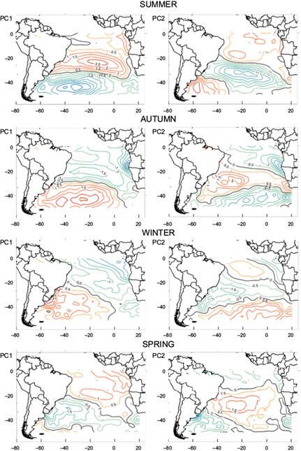
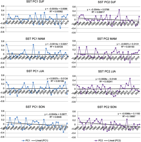
Fig. 2 Factor loadings of the first two principal components fields of SST anomalies for every season. The straight line corresponds to a linear trend with its formula.
Table I Linear trends of the SST factor loadings for every season.
| Principal component | Trend (ºC/year) | R |
| SST DJF PC1 | -0.0005 | 0.283 |
| SST DJF PC2 | -0.0044 | 0.261 |
| SST MAM PC1 | -0.0014 | 0.085 |
| SST MAM PC2 | -0.0007 | 0.043 |
| SST JJA PC1 | 0.0007 | 0.045 |
| SST JJA PC | 0.0008 | 0.049 |
| SST SON PC1 | -0.0049 | 0.291 |
| SST SON PC2 | -0.0066 | 0.396 |
Note: Coefficients in bold are significant with a 95% level of confidence.
For autumn, the first PC, with 25.6% of explained variance, shows two centers of highest variability placed in the northeastern and southwestern regions. The second PC, with 18.4% of explained variance, presents the maximum variability in the central region, including the Brazilian coasts, and centers with opposite sign to the south and northeastern areas of the basin. Both factor loadings time series present high variability with positive correlation coefficients prevailing over negative ones.
Regarding winter, the first PC presents 27.2% of explained variance and shows a dipole of maximum variability with two centers to the southwest and northeast of the basin. The second PC, with 11.3% of explained variance, shows highest variability in the center of the study area, including South America’s coasts, opposed to those located to the south and north. Positive correlation coefficients of PC2 dominate in the last 10 years of the record, explaining a higher number of years by that pattern.
Finally, for spring, the first PC presents 15.9% of explained variance and shows a pattern of highest variability in the central-western region opposed to the variability over the northeast and southwest regions. The second PC, with 13.3% of explained variance, presents a dipole of maximum variability located over the central and southwestern regions. PC2’s factor loadings present a significant negative trend with a 95% level of confidence, showing that SST’s variability during spring over the last years is mostly explained by cooler temperatures over the central region of the Atlantic basin and warmer waters over the Argentinian coasts. This pattern became more frequent by the end of the time record.
In all seasons, the first PCs show in general a dipolar behavior between the middle-high latitudes and the tropical Atlantic Ocean on the coasts of South America. Meanwhile, the second PCs are related to maximum variability in the central region of the Atlantic basin.
3.2 HGT1000 seasonal variability patterns
Figures 3 and 4, as well as Table II, show the first two HGT1000 anomalous PCs for every season along with their factor loadings. For summer, the first PC shows 37.5% of explained variance and presents a center of highest variability over the southern area of the basin. The second PC, with 11.9% of explained variance, shows two centers of maximum variability with opposite sign, located southwest and southeast of the region.
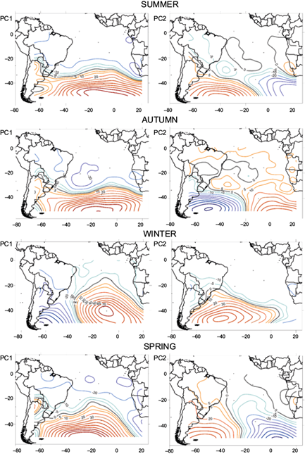

Fig. 4 Factor loadings of the first two principal components fields of HGT1000 anomalies for every season. The straight line corresponds to a linear trend with its formula.
Table II Linear trends of the HGT1000 factor loadings for every season.
| Principal component | Trend (gpm/year) | R |
| HGT1000 DJF PC1 | 0.0033 | 0.195 |
| HGT1000 DJF PC2 | -0.0045 | 0.268 |
| HGT1000 MAM PC1 | 0.0042 | 0.252 |
| HGT1000 MAM PC2 | -0.0048 | 0.285 |
| HGT1000 JJA PC1 | 0.0055 | 0.327 |
| HGT1000 JJA PC | -0.002 | 0.121 |
| HGT1000 SON PC1 | 0.0062 | 0.371 |
| HGT1000 SON PC2 | -0.0003 | 0.017 |
Note: Coefficients in bold are significant with a 95% level of confidence.
With regards to autumn, the first PC, with 39.4% of explained variance, presents a pattern of maximum variability over the southern region. The second PC, with 23.7% of explained variance, shows two centers of highest variability opposed to each other and located to the southeast and southwest of the Atlantic Ocean.
For winter, the first PC, with 37.9% of explained variance, shows two centers of maximum variability with opposite sign, over the southwest and central-east areas. In addition, the second PC, with 18.3% of explained variance, presents a center of highest variability over the central-west region. During these three seasons, PC1 factor loadings present a positive trend while PC2s a negative one, showing that HGT1000 variability is mostly explained by the PC1 pattern and the opposite pattern of PC2 shown in Figure 3 by the end of the record. Still, these trends are non-significant.
Finally, for spring, the first PC, with 41.9% of explained variance, presents a center of maximum variability located in the central-southern region and northern Argentina. The second PC, with 20.8% of explained variance, shows two centers of highest variability located over the eastern and western areas. A significant positive trend of PC1 factor loadings show that, over the second half of the record, the HGT1000 variability during spring is mostly explained by positive anomalies in middle and high latitudes.
With the exception of winter, the first PCs show a dipolar behavior between the middle-high and tropical latitudes while the second PCs reveal an east-west dipole over the middle-high latitudes over the Atlantic Ocean. In winter, however, the greatest HGT1000 variance is explained by the east-west dipole in middle-high latitudes.
3.3 Connection between SST and HGT1000
The interannual variability of the anticyclone and SST, specially over the coasts of the south Atlantic Ocean, have an influence over rainfall interannual variability. According to Garbarini et al. (2019), who studied rainfall variability connected to changes in the south Atlantic anticyclone, spring rainfall in Argentina shows the strongest signal whereas summer rainfall shows the weakest signal. Garbarini (2016) and Oliveri (2018) also found a correlation between climatic forcings related to SST and seasonal rainfall in Argentina.
In this work we intend to determine if the spatial variability pattern of SST can be associated to the possible strengthening and weakening of the South Atlantic Anticyclone. Table III shows the correlation between the first and second variability patterns of SST and HGT1000.
Table III Correlation between the first and second variability pattern of SST and HGT1000 over the Atlantic Ocean for summer, autumn, winter and spring.
| Summer | SST PC1 (28.5%) | SST PC2 (14.4%) |
| HGT1000 PC1 (37.5%) | -0.67 | -0.02 |
| HGT1000 PC2 (11.9%) | -0.24 | 0.41 |
| Autumn | SST PC1 (25.6%) | SST PC2 (18.4%) |
| HGT1000 PC1 (39.4%) | 0.22 | -0.47 |
| HGT1000 PC2 (23.7%) | 0.01 | -0.52 |
| Winter | SST PC1 (27.2%) | SST PC2 (11.3%) |
| HGT1000 PC1 (37.9%) | 0.45 | 0.03 |
| HGT1000 PC2 (18.3%) | 0.11 | -0.44 |
| Spring | SST PC1 (15.9%) | SST PC2 (13.3%) |
| HGT1000 PC1 (41.9%) | 0.04 | -0.57 |
| HGT1000 PC2 (20.8%) | 0.31 | -0.32 |
Notes: Coefficients in bold are significant with a 95% level of confidence; the explained variance of the variable is detailed in brackets.
HGT1000 patterns were analyzed in relation to those represented by the PCs of SST. In summer, the highest correlation between principal components was found between both the first PC of HGT1000 and SST anomalies. They have a correlation coefficient of -0.67 significant with a 95% level of confidence. This means that during these months, higher HGT1000 over the southern region is associated with warmer SST in the central and southern Atlantic Ocean, including the Argentinean coast, and cooler than normal SST to the north. The opposite pattern can also be present. The second significant correlation was found between HGT1000 PC2 and SST PC2 with a correlation coefficient of 0.41. This means that during summer, positive HGT1000 anomalies over the southwest region and negative over the southeast are associated with cooler SST over the central region of the basin and warmer SST over the Argentinean coasts. The opposite pattern can also be present.
During autumn, the highest significant correlation was found between the second PC of both variables, with a correlation coefficient of -0.52 with a 95% level of confidence. This means that during these months lower than normal HGT1000 in the southwestern region and higher than normal HGT1000 in the southeastern region, are connected with negative anomalies of SST in the center of the region, including the Brazilian coast, and positive anomalies to the north and south of the region. The opposite pattern is also possible. The second significant correlation was found between HGT1000 PC1 and SST PC2 with a -0.47 correlation coefficient. This shows that positive HGT1000 anomalies over middle and high latitudes are connected to warmer SST over the Argentinean coasts and south region of the basin, and cooler SST over the central-eastern region. The opposite pattern is also possible.
For winter, the highest significant correlation was found between the first PCs of both HGT1000 and SST with a 0.45 correlation coefficient. In this case, positive anomalies of HGT1000 over the southeast region and negative over the southwest (and therefore the presence of an east-west dipole) are connected to warmer SST in the central and southern Atlantic Ocean and cooler SST to the east and north of the study area. The opposite pattern can also be found. The second highest significant correlation found was between the second PCs of both variables, with a -0.44 correlation coefficient. This shows that positive HGT1000 anomalies over the southeast are connected to warmer SSTs over the central region and cooler to the south. The opposed pattern can also be present.
Finally, during spring, the only significant correlation was found between the first PC of HGT1000 and the second PC of SST and with a -0.57 coefficient. This means that negative anomalies of HGT1000 to the south are associated with warmer SST in the center of the region, and cooler SST to the south including the coast of Argentina. In addition to this, positive anomalies of HGT1000 to the south are connected to warmer SST in the southwestern South Atlantic Ocean, including Argentina, and cooler in the center of the study area.
4. Conclusions
The aim of this work is to analyze the connection between SST and geopotential height patterns in the South Atlantic Ocean. Regarding the general behavior of SST, the highest variance is explained by a dipolar behavior between the middle-high latitudes and the tropical Atlantic Ocean on the coasts of South America in all seasons. Meanwhile, the second PCs are related to maximum variability in the central region of the Atlantic basin.
Regarding the HGT1000 patterns, the highest variance is explained by a dipolar behavior between the middle-high and tropical latitudes and the second main pattern is an east-west dipole over the middle-high latitudes, in all seasons except winter. During this last season, the highest percentage of explained variance is associated with a zonal dipole over high latitudes.
When studying correlations between the principal components of both variables, we could observe that a pattern consisting of negative anomalies of SST over the southwestern region is related to different patterns of HGT1000 depending on the season. A similar behavior could be seen in spring and summer patterns. They both show that negative low-level geopotential height anomalies are associated with warmer SSTs in the central and northern parts of the region, and cooler temperatures to the south. An opposite pattern can be found during autumn and winter, when negative low-level geopotential height anomalies in the southwestern region are connected to warmer SSTs in the south area and cooler in the center of the basin.
Analyzing the behavior of the semi-permanent AH, an intensification during winter, meaning positive low-level geopotential height anomalies, is associated with warmer SST in the central and southern Atlantic Ocean and cooler SST to the east and north of the study area. Also, intensification during spring is connected to warmer SST in the southwestern South Atlantic Ocean, including Argentina, and cooler in the center of the study area.
We can detect that a percentage of the variability of the HGT1000 patterns can be explained by the SST patterns’ variability. There are many other processes that can also explain this variability. This study only shows that a part of this variability is related to the connection between both variables.

