


 text new page (beta)
 English (pdf)
 Article in xml format
 Article references
 Send this article by e-mail
 Cited by SciELO
  Similars in
SciELO
Similars in
SciELO 
 Permalink
1. Introduction
The Gulf of Mexico (GoM) is a large, transnational oceanic basin located in North America that is shared by Mexico, Cuba, and the United States. Mexico has 16 rivers that discharge directly into the GoM. Five of these rivers contribute most of the continental water that flows into the gulf, which totals ~220 × 109 m3 year-1 and represents around 90% of the net runoff from the Mexican side of the gulf (CONAGUA, 2014).
Stream flow is necessary to simulate nitrogen (nitrate and ammonium) loads, which are a product of anthropogenic activities and discharge directly into the ocean. The lack of daily discharge data from Mexican river mouths has resulted in several biogeochemical and oceanographic studies of the GoM (Martínez-López and Zavala-Hidalgo, 2009; Xue et al., 2013) using monthly (Milliman and Farnsworth, 2013; Dai, 2016), incomplete, or outdated discharge data from streams that flow into the gulf in their analysis.
The Soil and Water Assessment Tool (SWAT; Arnold et al., 1998) was used to model missing daily streamflow data. This model was chosen because of its ability to simulate hydrological and biogeochemical processes and its ability to efficiently handle and process all input data using Geographic Information Systems. A 25-yr simulation was performed for the four major basins: Usumacinta, Coatzacoalcos, Papaloapan, and Pánuco. In addition, a 17-yr simulation was performed for the Grijalva basin due to existing gaps in the available data for the calibration process.
2. Methods
2.1 Study area
The study region corresponds to a specific continental area delimiting the southern and western portions of the GoM. This region is formed by the Grijalva, Usumacinta, Papaloapan, Coatzacoalcos, and Tonalá watersheds in southern Mexico, as well as by the Pánuco watershed in northeastern Mexico (Fig. 1). The criteria used to select the study basins was based on the rate of the river discharge flowing into the gulf using historical data reported by CONAGUA (2017).
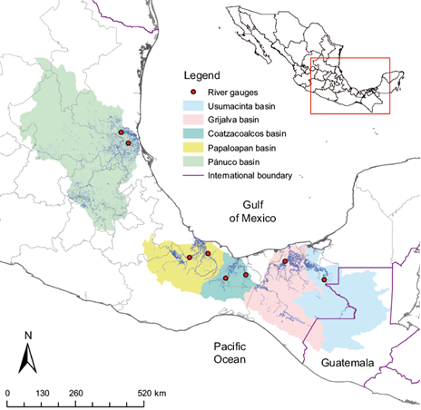
Fig. 1 Location of the studied basins and corresponding river gauges used for comparison and calibration.
Some selected basins are transnational, such as the Grijalva and Usumacinta basins, which extend into Guatemala (García-García and Kauffer-Michel, 2011). The Grijalva and Usumacinta watersheds cover a surface of 56 895 and 73 176 km2, respectively, and share a common river mouth located in the Mexican state of Tabasco. The highlands of these two basins present the highest annual precipitation values of all the analyzed zones (~4000 mm; Hinojosa-Corona et al., 2011). The elevations in the Grijalva and Usumacinta catchments vary from 0 to ~3600 masl. The dominant land uses for the Grijalva and Usumacinta catchments are agriculture and evergreen forest, respectively. Finally, four important dams are present within the Grijalva basin: La Angostura, Manuel Moreno Torres (Chicoasén), Nezahualcóyotl (Malpaso), and Peñitas (González-Villareal, 2009).
The catchments of the Coatzacoalcos (21 380 km2 extension) and Papaloapan (42 143 km2 extension) rivers span portions of the states of Veracruz, Oaxaca, and Puebla in southern Mexico. The average annual precipitation in this part of Mexico ranges between 1000 and 2200 mm (Ostos, 2004; Ponette-González et al., 2010). The elevations of these two catchments vary from 0 to ~2000 masl and the dominant land use in both areas is agriculture.
The Pánuco river watershed, which is separated from the previously described basins, is located in northeastern Mexico and covers an area of 147 367 km2. As a result of its extension, the greatest difference in average annual precipitation is present within the Pánuco watershed and ranges from 600 mm in the northern portion of the catchment to 1200 mm in the southern portion (Comrie and Glenn, 1998). The dominant land use in the Pánuco watershed is pasture land followed by mixed forest, savanna, and agriculture.
2.2 SWAT model
The SWAT model, developed at the Agricultural Research Service of the US Department of Agriculture (ARS- ), is a semi-distributed hydrological model that runs on both daily and monthly time steps (Arnold et al., 1998; Gassman et al., 2007; Saha et al., 2014a). It was chosen because of its ability to simulate flows, sediments, and nutrients in a closed basin. The SWAT model simulates the hydrological cycle based on the water balance equation:
where SW 0 and SW t are the initial and final soil water content, R day is the amount of precipitation, Q surf is the amount of surface runoff, E a is evaporation, W seep is the amount of water entering the vadose zone, and Q gw is the return baseflow. All variables on day i are in millimeters.
2.3 Databases
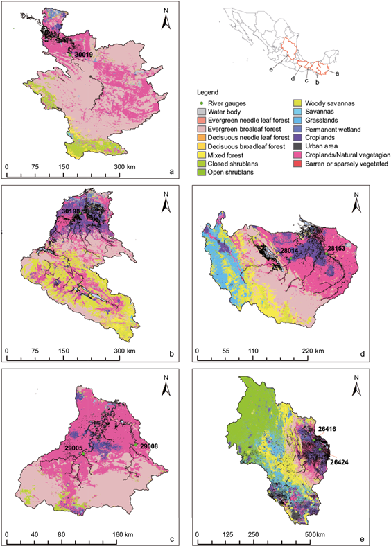
The model requires specific meteorological, topographic, land cover, and land use data for the study basins. All input data were integrated into the model via raster data sets, weather stations locations, and measured data files. The topography was obtained using an SRTM Digital Elevation Model (DEM; Jarvis et al., 2008) with a 90 m horizontal resolution. Meteorological data was obtained from Livneh et al. (2015), which has daily records of precipitation, maximum and minimum temperature, and wind speeds from 1950 to 2013 in North America with a 1/16º spatial resolution. Relative humidity and solar radiation data were obtained from the National Centers for Environmental Prediction (NCEP) Climate Forecast System Reanalysis (CFSR; Saha et al., 2014b) using the weather generator integrated into the SWAT model. To define land use (Fig. 2) we used the 500 m horizontal resolution product of the Moderate Resolution Imaging Spectro radiometer (MODIS) database distributed by the United States Geological Survey (USGS; Broxton et al., 2014). Soil information was obtained from the digital soil map of the world provided by the United Nations Food and Agriculture Organization (FAO, 2013). All observed data used for comparison, calibration and validation purposes in the present study were obtained from the Banco Nacional de Datos de Aguas Superficiales (BANDAS) database (CONAGUA, 2017), which contains daily discharge data from 2070 hydrometric stations.
2.4 Model setup
ArcSWAT (v. 2012.10.19) was used to facilitate the data entry, setup, and parametrization of the model in the present study. All basin watersheds were delineated automatically, which consisted of calculations of flow direction and accumulation using the DEM mentioned in Section 2.3. The selected outlets (i.e., points of discharge) in all basins were the ones located at the river mouths. Outlets were also added to match the location of river gauges. Reservoirs had to be added in the Grijalva basin in order to account for existing dams. Detailed information on dam operation was obtained from González-Villareal (2009). After delineating the watersheds, a hydrologic response unit (HRU) analysis was carried out based on soil, land use and slope (Table I).
Table I General configuration of the studied basins.
| Basin | HRUs | Sub-basins | Extension (km2) |
| Grijalva | 511 | 23 | 59755 |
| Usumacinta | 561 | 27 | 73075 |
| Coatzacoalcos | 219 | 15 | 21381 |
| Papaloapan | 347 | 20 | 42143 |
| Pánuco | 848 | 33 | 147367 |
HRU: Hydrologic response unit.
The simulation was carried out for two different periods: January 1, 1989 to December 31, 2013 for the Usumacinta, Coatzacoalcos, Papaloapan, and Pánuco basins and from July 7, 1997 to December 31, 2013 for the Grijalva basin. These periods were defined based on the available measured data. A spin-up period of 3 years (starting on1 January, 1986) was used in all simulations.
2.5 Model calibration, validation, and sensitivity analysis
Model calibration was conducted with an automatized technique using the Soil and Water Assessment Tool Calibration and Uncertainty software (SWAT-CUP 2012, v. 5.1.6; Abbaspour, 2011) and the SUFI-2 method (Abbaspour et al., 2004, 2007) for all calibrations. In SUFI-2, the uncertainty (referred as the 95% prediction uncertainty, 95PPU) is propagated using the Latin hypercube scheme (LHs) and calculated at the 2.5% and 97.5% levels for all variables (Schuol and Abbaspour, 2006). The model was calibrated and validated in monthly time steps; a total of 300 simulations were performed in each of the five iterations during the calibration. The calibration process took place for the period from 1989 to 2009 for the Usumacinta, Coatzacoalcos, Papalopan and Pánuco basins and from 1997 to 2013 for the Grijalva basin.
For the calibration process, we used the rules for parameter regionalization reported by Abbaspour et al. (2015). Based on these rules, we selected the threshold depth of water in shallow aquifer for baseflow to occur (GWQMN), the there-evaporation coefficient (GW_REVAP), the threshold depth of water in shallow aquifer for evaporation to occur (REVAPMN), the moisture condition II curve number (CN2), the soil available water capacity (SOL_AWC), the soil evaporation compensation coefficient (ESCO), and other parameters used in several studies (Moriasi et al., 2007), such as the maximum amount of water that can be trapped in the fully developed canopy (CANMAX), the effective hydraulic conductivity of the main channel (CH_K2), the plant soil-water uptake compensation factor (EPCO), the delay time for aquifer recharge (GW_DELAY), the aquifer percolation coefficient (RCHRG_DP), the soil depth (SOL_Z), and the surface runoff lag coefficient (SURLAG). For the Grijalva basin, parameters related to dam operation were also used; specifically, the hydraulic conductivity of the reservoir bottom (RES_K), the reservoir surface area when the reservoir is filled to the emergency spillway (RES_ESA), the volume of water needed to fill the reservoir to the principal spillway (RES_PVOL), the initial reservoir volume (RES_VOL), the maximum daily outflow for the month (OFLOWMX), the minimum daily outflow for the month (OFLOWMN), the average daily principal spillway release rate (RES_RR), and the lake evaporation coefficient (EVRSV). All the parameters used for all the calibrations are shown in Table II.
Table II Parameters used in all flow calibrations.
| Parameter | Unit | Method | Range |
| CN2 | - | r | -0.25 to 0.25 |
| ALPHA_BF | days | a | 0 to 1 |
| GW_DELAY | days | v | 0 to 500 |
| GWQMN | mm H2O | v | 0 to 5000 |
| CANMAX | mm H2O | v | 0 to 100 |
| CH_K2 | mm H2O/h | v | 0 to 500 |
| EPCO | - | v | 0 to 1 |
| ESCO | - | v | 0 to 1 |
| GW_REVAP | mm H2O/h | v | 0.02 to 2 |
| RCHRG_DP | - | v | 0 to 1 |
| REVAPMN | mm H2O | v | 0 to 500 |
| SOL_AWCa | mm H2O/mm | r | -0.25 to 0.25 |
| SOL_Za | mm | r | -0.25 to 0.25 |
| SURLAG | days | a | 0.05 to 24 |
| RES_Kb | mm/hr | r | 0 to 1 |
| RES_ESAb | ha | r | 1 to 3000 |
| RES_PVOLb | 104 m3 | r | 10 to 100 |
| RES_VOLb | 104m3 | r | 10 to 100 |
| OFLOWMXb | m3 s−1 | r | 0 to 2000 |
| OFLOWMNb | m3 s−1 | r | 0 to 1000 |
| RES_RRb | m3 s−1 | r | 0 to 1000 |
| EVRSVb | - | r | 0 to 1 |
aParameter adjusted depending on soil type; bParameters used only in the Grijalva basin. Methods: a: absolute, a given value is added to the existing parameter; r: relative, the existing parameter is multiplied by one plus a given value; v: replace, the old parameter is replaced by a new one.
Calibration performance was assessed using Nash-Sutcliffe efficiency (NS), the percentage bias (PBIAS), and the RMSE-observations standard deviation ratio (RSR) from the following equations:
where Q i obs is the observed discharge, Q i sim is the simulated discharge, and Q̅ sim is the mean of the measured data. Values of NS > 0.50 (Santhi et al., 2001), RSR < 0.70, and −25% ≤ PBIAS ≥ 25% in the statistical evaluators are necessary in order to consider a calibration successful, as established in the criteria provided by Moriasi et al (2007). The correlation factor (r) was also calculated to observe the lineal relationship between the observed and simulated signals from the following equation:
where x is the observed flow Q obs , y is the simulated flow Q sim , S xy is the covariance of the variables x and y, respectively, and S x and S y are the standard deviations of the corresponding variables. To validate the model, the same statistical estimators were calculated for the 2010 to 2013 period for all basins, with the exception of Grijalva basin that had insufficient available data to define a validation period.
According to Moriasi et al. (2007), the sensitivity analysis of the model can be estimated by changes in the outputs of the model in response to variations in different input parameters. A multiple regression analysis is used by the calibration software to obtain statistics for the sensitivity parameter. The significance of each parameter is evaluated with a t-test that yields the p-value (Abbaspour, 2011).
3. Results and discussion
In general, good calibrations were obtained in the study for the inland gauges. Figure 3 shows the observed and best signal flowmodel estimations, with values of NS > 0.50 and RSR < 0.70 for the Usumacinta, Coatzacoalcos, Papaloapan, and Pánuco basins, and PBIAS between ±5% and ±25% for all study basins, which according to Moriasi et al. (2007) are good fits for monthly time step calibrations. Furthermore, the correlation (r) between the observed and simulated signals for the basins was satisfactory for both monthly (0.76 ≤r ≤ 0.91) and daily (0.55 ≤ r ≤ 0.86) time scales.
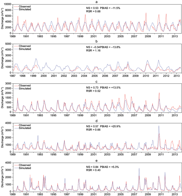
Fig. 3 Observed (red line) and simulated (blue line) discharges for the Usumacinta (a), Grijalva (b), Coatzacoalcos (c), Papaloapan (d), and Pánuco (e) rivers. Basins c, d, and e correspond to the 29005, 28153, and 26424 river gauges, respectively. All observed and simulated periods spanned from 1 January, 1989 to 31 December, 2013,with the exception of the Grijalva river period, which spanned from 7 July, 1997 to 31 December, 2013.
A brief explanation of the observed discharge signal and the corresponding best estimation signal are described below and presented in Table III. The observed mean discharge for the Usumacinta river was 2085.7 m3s−1, which was slightly lower than the simulated mean of 2457.7 m3s−1. The simulated flow ranged between 640 and 6105 m3s−1, which compares well with the observed limits of 156 and 7147 m3s−1 for the analyzed period and agrees with the values reported by Fuentes-Yaco et al. (2001) of 288 and 7442 m3s−1 for long-term historical data. The Grijalva basin is probably the most relevant of all study basins because it was possible to simulate an uninterrupted long-term discharge signal for the whole basin (Fig. 2b) that included the calibration point and the river mouth. The best simulation of the Grijalva basin showed values of 604.8 m3s−1 and 628.88 m3s−1 at river gauge 30198 for the observed and simulated discharges, respectively (Fig. 2b). On the other hand, the model showed a mean discharge of 1526.3 m3s−1 at the river mouth, which differs from the value of ~600 m3s−1 that has been widely used in previous oceanographic studies as the total amount of water that flows into the gulf from this basin. The Coatzacoalcos basin model showed a mean discharge of 397.44 m3s−1 compared with the observed discharge of 454.49 m3s−1 at river gauge 29005. The Papaloapan model simulated mean discharge of 663.62 m3s−1 and an observed mean discharge of 591.62 m3s−1 at river gauge 28014. Finally, the Pánuco basin model simulated a mean discharge of 429.2 m3s−1 and an observed mean discharge of 426.31 m3s−1 at river gauge 26424.
Table III Observed and simulated flows for the studied basin.
| Basin | Observed (m3s-1) | Simulated (m3s-1) |
| Usumacinta | 2085.7 | 2457.7 |
| Grijalva | 604.8 | 628.88 |
| Coatzacoalcos | 454.49 | 397.44 |
| Papaloapan | 591.62 | 663.62 |
| Pánuco | 426.31 | 429.2 |
All signals were in phase, which demonstrates the capability of the model to reproduce the runoff response of the basins despite differences in soil cover and land use in the southern basins compared with the Pánuco basin. The amplitude signals differed from one another depending primarily on the precipitation rate, which was due to basin location, and secondly on the extension of the basin. The Pánuco basin (Fig. 3e), which is the largest of the study basins, can be used to better understand this result. In the Pánuco basin, a mean discharge amplitude of ~430 m3s−1 and discharge peaks of ~2000 m3s−1 can be observed, which are similar to values of ~400 and ~1500 m3s−1 of the Coatzacoalcos basin, respectively (Fig. 3c). The similarity between the signals of the Pánuco and Coatzacoalcos basins is closely related to the differences in precipitation between the areas where the basins are located (Figs. 1, 2) and not to the extensions of the basins, as is the case for all four southern basins (Fig. 2a-d). Overall, there is a strong correlation between surface runoff and precipitation in the rainy season (June to October), with the peak events occurring in September (Fig. 4) in all basins.
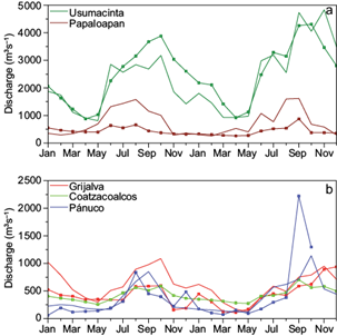
Fig. 4 Interannual discharge cycle spanning from 1 January, 2012 to 31 December, 2013 in all the studied basins. Solid and doted lines represent the observed and simulated signals, respectively.
Given that the simulation result is expressed by the 95PPU band, it cannot be compared to the observed signals using r, NS, or RSR. Instead, we used the P-factor and the R-factor (Abbaspour et al., 2004, 2007; Rouholahnejad et al., 2012) for comparisons. The P-factor is the amount of observed data within 95PPU and the R-factor indicates band thickness and is a measure of calibration quality (Rouholahnejad et al., 2012). The best fit for these parameters was obtained for the Pánuco basin (Fig. 5e) with a P-factor of 0.86 and an R-factor of 0.65.
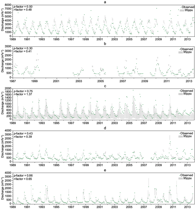
Fig. 5 Monthly observed flow (green dots) and the 95% prediction uncertainty (gray bars) for the Usumacinta (a), Grijalva (b), Coatzacoalcos (c), Papaloapan (d), and Pánuco (e) rivers. The calibration period spanned from 1 January, 1989 to 31 December, 2009 for all basins, with the exception of Grijalva basin, which was calibrated for the whole simulation period.
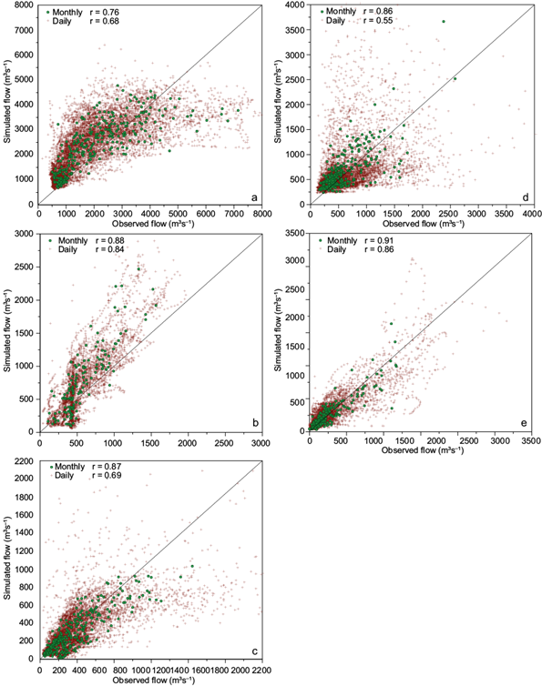
Fig. 6 Comparison between observed and simulated monthly and daily flows for the rivers (a) Usumacinta, (b) Grijalva, (c) Coatzacoalcos, (d) Papaloapan, and (e) Pánuco.
The results of the sensitivity analysis indicated that different basin models were sensitive to different parameters (p-values ≤ 0.05). The Grijalva basin model was most sensitive to REVAPMN, GWQMN, RCHRG_DP, ESCO, OFLOWMN and ESCO, while the Usumacinta basin model was most sensitive to RCHRG_DP, GWQMN, GW_REVAP, CN2 and SOL_AWC. The Coatzacoalcos basin model was sensitive to ALPHA_BF, GW_DELAY, CN2, and CH_K2 and the Papaloapan basin model was sensitive to GW_DELAY, ALPHA_BF, CN2, and SOL_AWC. Finally, the Pánuco basin was sensitive to CN2, ALPHA_BF, GW_REVAP, GWQMN, RCHRG_DP, and SOL_Z. The sensitivity analysis results indicate that all the generated models were sensitive to groundwater parametrization, followed by the moisture condition curve number (CN2). Our results provide valuable information that will improve parameter selection for the area in future studies.
4. Conclusion
Despite the dispersion between the observed and simulated daily flows in the Usumacinta, Coatzacoalcos, and Papaloapan watersheds, the model calibration presented satisfactory results for the analyzed basins. The greatest difference between the observed and simulated data was found in the Grijalva basin and was attributed to the incapacity of the model to reproduce large dams or reservoirs despite the availability of detailed dam operation data, which was also evident for the Papaloan basin where the Miguel Alemán dam is located. The daily data discrepancy between the observed and simulated flow, present in the Pánuco basin, may be associated with the extension of the basin and to the large differences in land use and soils present. In all basins, the calibration process showed that most of the models were sensitive to groundwater parameters. The results of this study indicate that underestimated discharge data has been used as the total net discharge flowing into the Gulf of Mexico for some rivers in previous studies due to the lack of available data, which is most evident for the Grijalva basin. Previously, total net river discharge data had been obtained from historical monthly climatologies or upriver gauges that are not located at river mouths where the total flow should be determined. It is also in the basin regions where the three main land-ocean interaction processes occur, which are contaminant and nutrient dispersion that is crucial for primary production; sediment transport that modifies coastal morphology, and the formation of fronts and baroclinic instabilities that are the product of salinity and temperature gradients. While the results of this study for the five studied basins are preliminary, they provide a solid basis for the improvement of future oceanographic and hydrological studies.

