text new page (beta)
 English (pdf)
 Article in xml format
 Article references
 Send this article by e-mail
 Cited by SciELO
  Similars in
SciELO
Similars in
SciELO 
 Permalink
1. Introduction
Over the last few decades, it has been observed that the Earth is experiencing a global warming, associated with the increase of extreme drought conditions, intense heat waves, floods, and changes in wind speed (Stott et al., 2004; Arango et al., 2012). In addition, it is expected that the average temperature will increase between 0.3 and 4.8 ºC worldwide (IPCC, 2014; Olaguer, 2016). The projections made for the 21st century indicate there will be a significant reduction of renewable surface and groundwater resources in most of the tropical dry regions, increasing competition between the different sectors that depend on water resources: agriculture, ecosystems, human settlements, energy industry and production (Karmalkar et al., 2011; Ospina et al., 2009a, b; Gay, 2000). According to Burger et al. (2016) and the IPCC (2014), the increases in terms of projected temperature will modify all aspects of food security, including the use and access to food and prices stability. These changes will be evident in all geographic scales (e.g., regional and local, high and low latitudes), being higher in low latitudes (IPCC, 2014). Climate models generate these climate projections based on greenhouse gas emissions (GHG).
The models included in the IPCC’s Fifth Assessment Report (AR5) (IPCC, 2014) consider four different Representative Concentration Pathways (RCPs), which are associated to GHG expressed in terms of CO2 equivalent (CO2 eq) for the year 2100. The RCP’s 6.0 and 8.5 indicate higher GHG (850 and 1370 ppm of CO2 eq, respectively) that could have disastrous impacts on the planet. While the scenarios with lower emissions, RCPs 2.6 and 4.5 (490 and 650 ppm CO2 eq., respectively) may cause fewer effects (IPCC, 2014). In the same way, RCPs project the following global temperature increases at the end of the 21st century: 0.3-1.7 ºC (RCP 2.6), 1.1-2.6 ºC (RCP 4.5), 1.4-3.1 ºC (RCP 6.0), and 2.6-4.8 ºC (RCP 8.5).
Global and regional climate models are the standard for producing climate change scenarios today (Bae et al., 2011; Jackson et al., 2011; Olsson et al., 2011; Kling et al., 2012; Gosling and Arnell, 2016). The last IPCC report considers the simulations from the climatic models from the Coupled Model Intercomparison Project Phase 5 (CMIP5). This project includes long-term simulations for a wide variety of variables such as rainfall and temperature that were projected by different research centers. Each climatic model run is based on the description of RCPs; however, the projections for the proposed scenarios differ significantly between models (Arango et al., 2012). Some studies make ensembles, based on assumptions about the relative weight given to each scenario (Manning et al., 2009; Christierson et al., 2012; Liu et al., 2013). In this way, an ensemble mean simplifies the information given by climate models, producing a single future scenario, and enables assessment of the impacts of climate change on a system of interest such as water resources.
Most of the water resources assessments have used hydrological models applying the delta change factor methodology or the change factor methodology (Anandhi et al., 2011). This method creates different scenarios, applying the climate changes projected by a climatic model to an observed baseline climate. Several approaches have been developed for the construction of scenarios at basin or local scale (Fowler et al., 2007). This includes the scale reduction techniques using regional climate models and a variety of statistical approaches (Fu et al., 2013).
Systematic assessments of different methods have demonstrated that the estimated impacts could depend on the approach employed to reduce the scale of the climate model data. Additionally, the uncertainty range between the approaches of scale reduction can be as wide as the range between different climatic models (Quintana et al., 2010; Chen et al., 2011). Another approach for the impact assessment is an inverse technique (Cunderlik and Simonovic, 2007), which begins identifying the hydrological changes that would be critical for a system. Then, it uses a hydrological model to determine which meteorological conditions cause the changes (Jiménez et al., 2014).
Sometimes the ensemble mean is used in impact assessments. This can be considered as a simplified scenario. However, this technique does not allow detecting each scenario effect, entailing additional uncertainty. This is particularly the case of the Reliability Ensemble Averaging (REA), a multi-model and multi-scenario ensemble, which is currently widely used by institutes and research centers. REA was presented by the Instituto de Hidrología, Meteorología y Estudios Ambientales (Institute of Hydrology, Meteorology and Environmental Studies, IDEAM) of Colombia during the United Nations Framework Convention on Climate Change. Projections using this aproach suggest that by the end of this century, the annual average temperature could increase by 2.14 ºC and the annual average precipitation could decrease between 10 and 30 % in many regions in Colombia (IDEAM, 2015). These climatic changes will modify the hydrological cycle on a large scale and will significantly affect the most vulnerable systems that depend on hydric resources, including agricultural systems, since water availability and sources, aquifers, and precipitations will be limiting factors (FAO, 2008). One of the limitations in this kind of ensemble is that the results are spatially coarse, thus it is not possible to propose or design precise local and/or regional adaptation strategies.
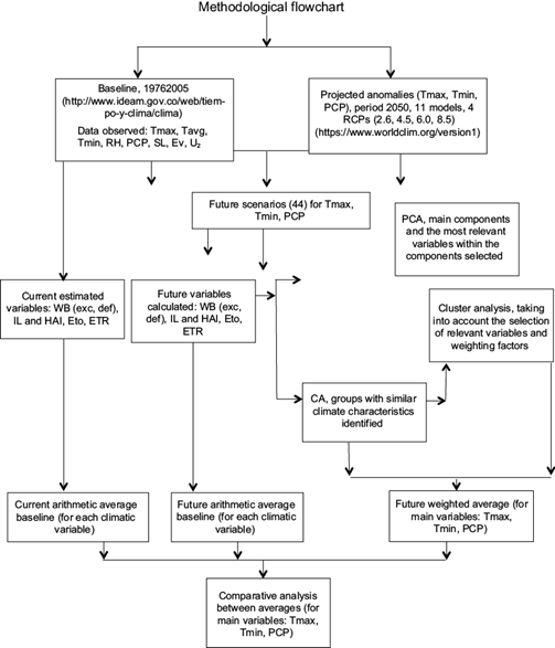
In this study, the effects of all scenarios are evaluated in an issue of interest: the availability of water for agricultural purposes. Thus, the aim of this study was to generate an ensemble mean of climate scenarios that take into account weighting factors obtained through a multivariate statistical analysis. The weighting factors consider the most negative effects on the availability of water resources projected by different climate change scenarios. This method generates a single weighted average scenario which provides information on the most adverse effects. Additionally, this ensemble mean could help policymakers and regional and local stakeholders to implement better adaptation measures and to use more efficiently the local natural, economic, and human resources.
2. Methodology
2.1. Selection of the study area and collection of information
The study area is the municipality of Nilo (Cundinamarca) due to its relevance to the project Mejoramiento de la Tecnología de Producción de Cacao en las Provincias de Rionegro y Alto Magdalena (improvement of the cocoa production technology in the Rionegro and Alto Magdalena provinces), Cundinamarca, conducted by the Universidad Nacional de Colombia.
2.1.1 Study area
In order to describe the climate conditions in the study area, a baseline was established, and certain information was collected from the IDEAM’s network of weather stations. The precipitation (PCP) baseline was established using information of the pluviometric weather station in Nilo, Cundinamarca (4º 18’ 21.2” N, 74º 38’ 55.2” W) for the years 1976-2005. Since the municipality has no weather stations, it was necessary to have at least an approximation of its climatic conditions using information from other stations close to the municipality. For other variables (relative humidity [Rh], evaporation [Ev], sunlight [SL], temperatures [T]), historical data was collected from the weather station of Melgar, Tolima (4º 12’ 44” N, 74º 38’ 12.6” W) for the years 1976-2005. It is worth noting that the data records of Melgar were used because it is the weather station with meteorological information closest to the area of study. Additionally, both weather stations have similar climatic characteristics in terms of temperature and precipitation.
2.1.2. Calculation of the potential evapotranspiration and analysis of the current water balance
To calculate variables related to the analysis of water availability for agricultural purposes, potential evapotranspiration (ETo) was evaluated (Appendix A.1). ETo was calculated using the established baseline and the Penman-Monteith method (Allen et al., 2006) recommended to determine the ETo from other climatic parameters (Eq. 1).
where ETo is the potential evapotranspiration (mm day-1), Δ is the slope of the saturated vapor pressure curve, Rn is the net radiation at the crop surface (MJ m-2 day-1), G is the soil heat flux (MJ m-2 day-1), γ is the psychometric constant (KPa × ºC-1), T is the average temperature (ºC), U 2 is the wind speed (m s-1), and e s - e a represents the vapor pressure deficit (KPa).
Then water balance was estimated taking into account the precipitation and potential evapotranspiration to determine deficits (Def), excess (Exc), real evapotranspiration (ETR), soil water storage, and change in soil water storage for the current conditions. Detailed information about the methodologies used is available in Ospina et al. (2017).
Similarly, the phytoclimatic indexes of aridity were obtained: Lang’s index (precipitation/Taverage) and hydric availability index (Eq.2).
where ETR is the real evapotranspiration, Exc is the excess, and ETo is the potential evapotranspiration.
2.2 Generation of future scenarios
2.2.1 Model scenarios
In order to generate future scenarios, the anomalies projected for precipitation and the minimum and maximum temperatures were obtained from 11 general circulation models (Table I).
Table I Models used for the climatic projections in this study.
| Model | Code | Model | Code |
| BCCCM1-1 | BC | ROC-ESM-CHEM | MI |
| CCSM4 | CC | MIROC-ESM | MR |
| GISS-E2-R | GS | MIROC5 | MC |
| HadGEM2-AO | HD | MRI-CGCM3 | MG |
| HadGEM2-ES | HE | NorESM1-M | NO |
| IPSL-CM5A-LR | IP |
Additionally, four scenarios of GHG were considered: RCPs 2.6, 4.5, 6.0 and 8.5. Climate projections have a resolution of 5 min for the future period 2070, which are available at: http://www.worldclim.org/cmip5_5m. A geostatistical software (ArcMap) was used to display the climate variables of the study area.
2.2.2 Projection
The projected anomalies were added to the baseline climatology, resulting in 44 future climate scenarios (11 models 4RCPs) for each climatic variable (precipitation, Tmax and Tmin). This projects were used to calculate the indices described in sectrion 2.1.2 (see Appendix A.2).
2.3. Multivariate analysis
The results of the annual climatic variables obtained in the previous phase were subjected to principal component analysis (PCA) of standardized variables and cluster analysis (CA) using the Ward’s method and Euclidean distance. The Ward’s method is a hierarchical procedure where two clusters are joined at each step, obtaining the smallest increase of the sum of squares. This generates groups, which minimizes intra-group dispersion in each binary fusion (Murtagh and Legendre, 2014). Additionally, Unal et al. (2003) considered this method to be the most appropriate one to produce acceptable results in the case of the climatic zoning of Turkey. Further, they argued that similar results are often found in climatological studies. Therefore, Ward’s method is used for the methodology proposed in this study.
PCA allows selecting representative linear combinations from the original variables and shows the most relevant variables in each component related to hydrological resources and their direct or opposite relationship. CA allows differentiating groups with different climatic conditions. The analysis was performed using the software Statgraphics Centurion XV.II.
Multivariate analysis allowed clustering the scenarios that present differences regarding their climatic projections, as mentioned above, which also enabled to propose weighting factors for each group according to the prevention and/or mitigation criteria established by the system in question (in this case, hydric resources).
2.4. Proposal of management and ensemble of scenarios
A weighted average scenario was computed, since the water resource is a limiting factor for cultivation in the area of study (classified as a semi-arid zone and located in the appropriate lower limit in the hydric availability index); also, to have a scenario with a certain degree of certainty (where adaptation strategies can be proposed and designed). This average was proposed for the main climatic variables (PCP, Tmax, Tmin and Tavg), where the greatest weight will be given to future scenarios that project a higher decrease in precipitation and a higher increase in temperature. This will be evaluated because these two variables significantly affect the aridity and the parameters involved in the water balance of a region and, according to the PCA, they were the most relevant variables.
The weight of the elements of each cluster was determined by finding the average range of the variable of interest in each cluster, obtained similarly as in several non-parametric statistical methods (Conover, 1999). The proposed ensemble takes into consideration the weight of the variables, so the most negative impacts on the system can be specified according to the projections for all future scenarios.
3. Results and discussion
According to the baseline obtained from the historical data of the meteorological stations mentioned above (Table II), it was found that the study area had an annual average temperature of 26.5 ºC, a minimum temperature of 21.4 ºC, a maximum temperature of 31.6 ºC, and an annual precipitation of 1292.0 mm. According to Lang’s index (IL = 48.1) and the hydric availability index, it is a humid zone with vast grasslands, appropriate for agricultural crops to a limited extent (HAI = 90.7).
Table II Baseline climatic variables in the study area.
| Var/month | Jan | Feb | Mar | Apr | May | Jun | Jul | Aug | Sep | Oct | Nov | Dec | Sum/avg |
| PCP (mm) | 64.9 | 102.5 | 124.4 | 136.8 | 163.7 | 78.4 | 33.2 | 24.5 | 101.0 | 190.8 | 153.4 | 118.6 | 1292.0 |
| Tmax (ºC) | 32.1 | 32.1 | 32.2 | 31.9 | 31.7 | 31.7 | 31.6 | 31.9 | 31.8 | 31.0 | 30.8 | 31.0 | 31.6 |
| Tmin (ºC) | 21.2 | 21.3 | 21.4 | 21.1 | 20.9 | 20.9 | 21.8 | 22.1 | 22.0 | 21.2 | 21.1 | 21.2 | 21.4 |
| Tavg (ºC) | 26.7 | 26.7 | 26.8 | 26.5 | 26.3 | 26.3 | 26.7 | 27.0 | 26.9 | 26.1 | 26.0 | 26.1 | 26.5 |
| SL (h day-1) | 6.7 | 6.1 | 5.4 | 5.4 | 5.7 | 6.0 | 6.4 | 6.4 | 6.2 | 6.1 | 6.1 | 6.4 | 6.1 |
| RH (%) | 66 | 64 | 66 | 69 | 71 | 71 | 66 | 62 | 63 | 66 | 68 | 65 | 66.4 |
| Ev (mm) | 165 | 159 | 164 | 140 | 139 | 151 | 195 | 227 | 190 | 158 | 131 | 141 | 163.4 |
| U2 (m s-1) | 0.20 | 0.33 | 0.40 | 0.39 | 0.28 | 0.46 | 0.59 | 0.43 | 0.19 | 0.21 | 0.16 | 0.06 | 0.3 |
PCP: precipitation; Tmax: maximum temperature; Tmin: minimum temperature; Tavg: average temperature; SL: sunlight; RH: relative humidity; Ev: evaporation; U2: wind speed
Figure 1 illustrates the behavior of the main variables. Figure 1a shows the temperatures of the study area, which are higher in July, August, and September in comparison to other months. As shown in figure 1b, the PCP vs. Ev ratio suggests the condition of the water resource is practically deficient throughout the year, and water availability is scarce. This was confirmed by estimating the water balance.

Fig. 1 Annual behavior of variables. (a) Maximum temperature (Tmax), minimum temperature (Tmin) and average temperature (Tavg) for Nilo, Cundinamarca. (b) Precipitation (PCP) vs. evaporation (Ev) in Nilo.
Considering the values reported in Table II, the water balance was estimated for the current conditions, determining ETR, Exc, Def, storage and change of soil water, replacement and usage of the water stored in the soil (see Table III).
Table III Current water balance in Nilo, Cundinamarca.
| Variable | Jan | Feb | Mar | Apr | May | Jun | Jul | Aug | Sep | Oct | Nov | Dec | Sum/avg |
| PCP | 64.9 | 102.5 | 124.4 | 136.8 | 163.7 | 78.4 | 33.2 | 24.5 | 101.0 | 190.8 | 153.4 | 118.6 | 1292.0 |
| ETo | 112.9 | 106.0 | 117.2 | 111.7 | 111.1 | 107.4 | 117.1 | 121.3 | 115.8 | 115.3 | 104.4 | 104.6 | 1345.0 |
| ∆ | -48.0 | -3.5 | 7.1 | 25.1 | 52.6 | -29.0 | -83.9 | -96.8 | -14.8 | 75.5 | 48.9 | 14.0 | |
| S | 52.0 | 48.5 | 55.6 | 80.7 | 100.0 | 71.0 | 0.0 | 0.0 | 0.0 | 75.5 | 100.0 | 100.0 | |
| Def | 0.0 | 0.0 | 0.0 | 0.0 | 0.0 | 0.0 | 12.9 | 96.8 | 14.8 | 0.0 | 0.0 | 0.0 | 124.5 |
| Exc | 0.0 | 0.0 | 0.0 | 0.0 | 33.2 | 0.0 | 0.0 | 0.0 | 0.0 | 0.0 | 24.4 | 14.0 | 71.6 |
| ∆S | -48.0 | -3.5 | 7.1 | 25.1 | 19.3 | -29.0 | -71.0 | 0.0 | 0.0 | 75.5 | 24.5 | 0.0 | |
| ETR | 112.9 | 106.0 | 117.2 | 111.7 | 111.1 | 107.4 | 104.2 | 24.5 | 101.0 | 115.3 | 104.4 | 104.6 | 1220.4 |
| Condition | U | U | R | R | R | U | U | - | - | R | R | - |
PCP: precipitation; ETo: evapotranspiration, ∆: difference between P and ETo; S: storage; Def: deficit; Exc: excess; ∆S: change in the storage; ETR: real evapotranspiration; U: use of soil water; R: replenishment of water in the soil.
4. Future scenarios and multivariate analysis
After obtaining the anomalies of the most relevant variables (i.e., precipitation and temperature), by using the scenarios studied and elaborating future scenarios from the baseline, the water balance and the other indexes and parameters related were estimated based on future climate change scenarios. Appendix A.2 shows the annual values of the variables and parameters calculated for the scenarios projected to 2070, which are the input values or database in the multivariate analysis.
Some scenarios only project an increase of approximately 1 ºC and others an increase of approximately 5 ºC (see Appendix A.2). Also, some scenarios estimate an increase in precipitation of about 14%, while other projects a decrease of approximately 37%. This behavior is also the similar to the rest of the variables analyzed, which means that there is a high level of uncertainty when trying to identify the most likely future scenario to design and manage a system. This suggests that it could be useful to manage and generate ensemble scenarios upon which adaptation strategies can be proposed and designed for the system being studied.
The principal components analysis suggested the selection of two components with eigenvalues equal to or greater than 1.0, which explain 86.7% of the variability in the original data (see Fig. 2).

Table IV shows the weight of the variables in each component. It is observed that precipitation and indexes related with this variable (IL, Def, HAI) hold greatest weights in the first component, while temperature and parameters related thereto, such as RH and ETo, have greatest weights in the second component. This suggests that the weighting should be conducted on these input variables during the water resource availability analyses. Moreover, four clusters were created from 44 scenarios in the cluster analysis (see Fig. 3). The clusters are groups with similar characteristics or climate conditions.
Table IV Weights of hydrological variables for each component.
| Component | Def | ETo | ETR | Exc | RH | HAI | IL | PCP | Tmax | Tavg | Tmin |
| 1 | -0.419 | -0.009 | 0.421 | 0.29 | -0.063 | 0.429 | 0.43 | 0.435 | 0.021 | 0.015 | 0.019 |
| 2 | -0.063 | -0.411 | -0.015 | -0.03 | 0.433 | 0.04 | 0.07 | -0.023 | -0.448 | -0.475 | -0.454 |
Def: deficit; ETo: evapotranspiration; ETR: real evapotranspiration; Exc: excess; RH: relative humidity; HAI: hydric availability index; IL: Lang’s index; PCP: precipitation; Tmax: maximum temperature; Tavg: average temperature; Tmin: minimum temperature.

Table V shows the number of members (scenarios) in each group and the centroids or averages of the variables in each group. For example, cluster 3 projects the largest decrease in precipitation (874.743 mm) and contains seven scenarios. In consequence, this variable will have the greatest weight in these scenarios, distributed among its members. Meanwhile, cluster four projects an increase in precipitation (1314.08 mm), thus having a lower weight distributed among its eight members. Decrease and increase precipitation are analyzed based on current precipitation (1292.0 mm, see Table II).
Table V Summary of clusters and centroids.
| Cluster | Members | Percentage | Def | ETo | ETR | Exc | RH | HAI | IL | PCP | Tmax | Tavg | Tmin |
| 1 | 22 | 50.00 | 294.518 | 1395.4 | 1100.88 | 0.363636 | 64.3318 | 78.9091 | 38.6759 | 1101.25 | 33.8909 | 28.4909 | 23.0773 |
| 2 | 7 | 15.91 | 287.757 | 1429.86 | 1142.12 | 7.12857 | 59.3 | 80.03 | 38.3243 | 1149.27 | 35.4286 | 30.0286 | 24.6143 |
| 3 | 7 | 15.91 | 525.857 | 1400.6 | 874.743 | 0.0 | 62.5143 | 62.4571 | 30.4586 | 874.743 | 34.0571 | 28.7429 | 23.4 |
| 4 | 8 | 18.18 | 191.013 | 1389.53 | 1198.53 | 115.538 | 62.5875 | 88.3013 | 45.7113 | 1314.08 | 34.1 | 28.725 | 23.3875 |
Def: deficit; ETo: evapotranspiration; ETR: real evapotranspiration; Exc: excess; RH: relative humidity; HAI: hydric availability index; IL: Lang’s index; PCP: precipitation; Tmax: maximum temperature; Tavg: average temperature; Tmin: minimum temperature.
Similarly, temperatures were also weighted, giving greater weight to thosse variables in the clusters that project higher temperatures (cluster 2) and vice versa.
To determine the weight of the elements in each cluster, first the average range of the variable of interest, which indicates the difference (or no difference) between the medians of the groups, was determined. For purposes of illustration, PCP was selected as variable of interest, and it was obtained similarly as the ranges allocated in some parametric tests based on ranges. As shown in table VI, column 3, cluster 3 obtained the lowest average range, which should hold a greater weight because it contains the scenarios that project lower precipitation and consequently it is the group with the major negative impact on the system being studied (water availability). In this case, the inverse of the percentage relative average range was used (the inverse range of a group of interest with respect to the sum of the inverse of the total ranges; column 5), giving a greater weight to cluster 3 (69.1 %), followed by clusters 1, 2 and 4 in accordance to the logic of the criterion established in the methodology (section 4).
Table VI Weighting factors to obtain the PCP ensemble.
| Cluster | Cluster elements | Average range | Inv_average range | Inv_relative average range (%) | % cluster elements | Weighting factor |
| 1 | 22 | 21.2 | 0.047 | 13.0 | 50.0 | 0.26 |
| 2 | 7 | 25.4 | 0.039 | 10.9 | 15.9 | 0.68 |
| 3 | 7 | 4.0 | 0.250 | 69.1 | 15.9 | 4.34 |
| 4 | 8 | 39.6 | 0.025 | 7.0 | 18.2 | 0.38 |
| Sum | 44 | 0.362 | 100.0 | 100.0 |
Column 4 = 1/cluster value column (3); column 5 = [cluster value column (4)*100]/∑(4); column 7 = cluster value column (5)/cluster value column (6).
In this case, the greatest negative impact is associated with low precipitation, given that the study region is characterized by being a zone tending to aridity. Agricultural production systems have high water resource requirements; however, if a region has climatic and hydrological characteristics that conduce to wet zones with excess of water, the greatest negative impact would be given by scenarios that project an increase in precipitation. Thus, an advantage of this study is that it weighs scenarios according to the climatic characteristics of each zone and productive system expected to be evaluated. In terms of temperatures, a direct average range (percentage) was implemented, because a wider average range contains the scenarios that project a higher increase in temperatures, thus having a negative impact on water availability.
Finally, according to the percentage average ranges (or their respective inverses), the cluster weights are distributed according to the percentage of the elements in each group (column 6) to obtain the final weighting factor (column 7).
Following the proposed methodology, the weighting factors for the temperatures ensemble were identified, which are summarized in Table VII.
Table VII Weighting factors for the ensemble of Tmax, Tavg and Tmin.
| Cluster | Element | Weighted_Tmax | Weighted_Tavg | Weighted_Tmin |
| 1 | 22 | 0.36 | 0.34 | 0.34 |
| 2 | 7 | 2.46 | 2.45 | 2.44 |
| 3 | 7 | 1.35 | 1.38 | 1.39 |
| 4 | 8 | 1.17 | 1.22 | 1.23 |
| 44 |
Going back to the precipitation example, Table VIII shows the monthly baseline (BL), the arithmetic average (AA) and the weighted average (WA) of the precipitation projected by future scenarios. Figure 4a illustrates the monthly behavior of all scenarios, while figure 4b illustrates the BL, AA and WA.
Table VIII Current and future precipitation according to the future scenarios ensemble.
| Month | Jan | Feb | Mar | Apr | May | Jun | Jul | Aug | Sept | Oct | Nov | Dec | Sum | % change |
| BL | 64.9 | 102.5 | 124.4 | 136.8 | 163.7 | 78.4 | 33.2 | 24.5 | 101.0 | 190.8 | 153.4 | 118.6 | 1292.0 | - |
| AA | 62.4 | 121.5 | 104.7 | 115.0 | 156.6 | 56.5 | 27.4 | 12.8 | 87.6 | 150.1 | 114.4 | 102.6 | 1111.5 | -14.0 |
| WA | 45.5 | 97.1 | 95.3 | 113.8 | 146.4 | 49.5 | 24.7 | 11.7 | 77.5 | 133.9 | 92.6 | 76.7 | 964.8 | -25.3 |
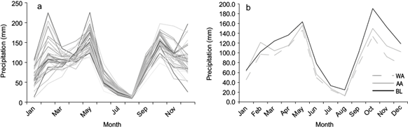
Fig. 4 (a) Future scenarios of precipitation for all the models by 2070. (b) Behavior of precipitation baseline (BL), arithmetic average (AA) and weighted average (WA) by 2070.
In Table VIII and figure 4b, the WA projects a larger decrease (-25.3%) in precipitation than in the AA (-14.0%), decreasing from the current precipitation of 1292.0 mm yr-1 to 936.5 mm and 1111.5 mm, respectively. This is consistent with our interest of finding a future scenario that considers all the scenarios and the logic of preventing the most negative impacts. This allows to propose and/or design adaptation strategies with a good level of certainty to prevent the most negative effects on water availability, which will also influence the hydric requirements of agricultural systems.
According to IDEAM (2015), precipitation will change by approximately -10 % and 10% in several municipalities of the Cundinamarca department. The study area, Nilo, will be within this range of change. In this case, the differences shown resulted from the methodology proposed in this research, including the analysis at a local scale and a weighted ensemble according to the most important unfavorable effects. On the other hand, the REA ensemble presented by IDEAM contemplates a regional geographic scale. Additionally, this ensemble is not based on the negative effects that each of the climatic scenarios could have on the studied system.
According to Räisänen (2007), normally projections have better performance if they are analyzed at larger scales. Mahlstein and Knutti (2010) argue that when a region is too small, the models may not agree with their projections. However, they claim that if the region is too large, the changes will be diffused and the information will be lost because different climate regimes are being averaged together. For example, averaging positive and negative changes in precipitation will result in a small net change. These authors recommend not to analyze too extensive regions because the information provided is not useful for evaluating local impacts, since it is unlikely that the regional average represents local changes. This is the case of changes in precipitation between -10 and 10% projected by the REA ensemble for the study area according to IDEAM, while the ensemble proposed in this study is useful to evaluate the impacts of climate change in a system at the local level.
Figure 5a, b, c illustrates the monthly behavior of temperatures and ensembles obtained.
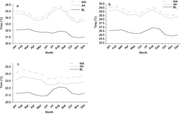
Table IX summarizes expected changes according to the AA and the WA in relation to the baseline or current condition of Tmax, Tavg and Tmin. Similarly to PCP, it can be observed that temperatures obtained with the WA have a higher increase than temperatures estimated with the AA. For example, the AA projects a change of 2.6 ºC Tmax with respect to the current temperature (Table IX, column 3), while the WA projects a change of 2.9 ºC (i.e., 0.3 ºC more). Therefore, a future scenario of temperature emerges again, enabling to conduct a water availability analysis based on the logic of preventing the most negative impacts as mentioned above. In this regard, by the end of the century, temperatures in the Cundinamarca department will increase by 2.3 ºC with respect to current temperatures. Temperature changes will particularly occur in the province of Alto Magdalena, where the current study was conducted (IDEAM, 2015).
Table IX Expected changes of temperature for the year 2070 according to the proposed ensembles.
| Tmax | Change (Tmax) | Tavg | Change (Tavg) | Tmin | Change (Tmin) | |
| WA | 34.6 | 2.9 | 29.2 | 2.7 | 23.8 | 2.5 |
| AA | 34.2 | 2.6 | 28.8 | 2.3 | 22.9 | 1.6 |
| BL | 31.6 | - | 26.5 | - | 21.4 | - |
Finally, IDEAM (2015) states that the main effects for the Cundinamarca department can occur in the agricultural sector due to the accentuated changes in temperature, as well as the persistence of pests associated with increased precipitation in the evaluated areas. Thus, the weighted average scenarios for PCP and temperature could be used as input variables to conduct different studies and analyses related to future climatic conditions in a region. These analyses could be water balance and the hydric requirements of agricultural systems within the study area, which are beyond the scope of this proposal and, therefore, will be presented in a further study.
5. Conclusions
The proposed methodology is easy to adopt, enabling the removal of subjectivity and uncertainty in these types of analyses to a certain extent. Additionally, it is a contribution to the development of future change scenarios.
As expected, the PCA suggests that the input variables for PCP, Tmax, Tavg, and Tmin are enough to elaborate an ensemble of future scenarios, upon which it is possible to conduct the required supplementary analyses. In this case, with respect to the water availability for agricultural purposes, which simplifies the calculations by reducing the dimensionality of the original dataset.
It is recommended that the weighted average is used to analyze the effects of climate change on the availability of water resources, in order to address the most negative effects. Therefore, each and every one of the projections for the study area is taken into account. However, this does not mean that any methodology that exhibits excessively extreme projections can be useful. Only those methodologies whose results are within the range exposed in the scenarios evaluated would be considered.
The proposed methodology not only applies to the assessment of climate change and how it affects water availability, but it also applies to many other systems, activities, or elements of interest. This method considers the most adverse or most beneficial effects according to the characteristics and particularities of the regions and/or systems evaluated.
Additionally, the use of the weighted average allows designing and proposing appropriate adaptation and/or mitigation strategies with a certain level of certainty, making the use of economic and human resources more efficient and effective.