


 text new page (beta)
 English (pdf)
 Article in xml format
 Article references
 Send this article by e-mail
 Cited by SciELO
  Similars in
SciELO
Similars in
SciELO 
 Permalink
1. Introduction
The aim of this research is to analyze the fractal behavior of rainfall events in a semiarid region located in Baja California, northwestern Mexico. Two analyses were performed to: (1) find a relation with climatological distribution, altitude, average temperature and average annual rainfall, and (2) compare different scales for the same time series. In order to achieve this goal, 92 climate stations with at least 30 yrs of records were analyzed; subsequently, using the Hurst exponents, a spatial and temporal analysis was carried out in order to compare it with the previously mentioned variables. The results could help analyzing the effects of climate change in this region.
It is well known that rainfall, being a random variable and part of a complex and chaotic system (Xu et al., 2015), evolves during time and space and exhibits extreme variability (Brunsell, 2010; Gires et al., 2014), as well as temporal trends (Shi et al., 2014), which also implies that these two dimensions are not mutually independent. It has been also found that the evolution ratio of rainfall is invariant through time and space in a dynamic scale, and that over wide ranges, atmospheric spatial variability can be well described (Pinel et al., 2014). Rainfall events are very erratic at short and large temporal and spatial scales (Millan et al., 2011). According to Zhang et al. (2013), rainfall extreme events have become more frequent and intense under global warming conditions, causing an increase in the number of days with extreme rainfall events; therefore studying the spatial correlation structure exhibited by rainfall measurements can provide useful results for understanding the effects produced by the interaction between meteorological patterns (Sirangelo and Ferrari, 2014). The statistical structure dependence of rainfall in space and time can be analyzed with a single parameter that studies its persistence (Venugopal et al., 1999). A research conducted in India proved that regional climatological models were not capable of adequately predicting local weather since they use average values; therefore, models that study the internal structure of the random variable are required (Rangajaran and Sant, 2004). The foundation of this statement is that extremely variable fields, such as rainfall, involve multiple scales and dimensions, being these two characteristics present in intense regions (Lovejoy et al., 1987). It has been confirmed that rainfall is a part of many factors involved in climate change which are characterized by persistence in the long term (Fluegeman and Snow, 1989). Hydrological data sets, such as rainfall, are constituted of complex fractal geometry which is complicated to represent using classical stochastic methods (Huai-Hsien et al., 2013). However, trying to study a single random variable at different scales turns out to be very complex, along with the fact that autoregressive methods can produce certain errors (Svanidze, 1980); hence, a new and revolutionary approach has emerged (Sivakumar, 2000) that has proven to be much more effective than classical autoregressive methods (Caballero et al., 2002; Nunes et al., 2011; Akbari and Friedel, 2014).
Mandelbrot (1967)) introduced the concept of a fractal in terms of self-similar statistic; this concept revolves around the idea that the shape of an object does not define its size. Mandelbrot defined fractals as objects that possess a similar appearance when observed at different scales, having details even at small arbitrary scales; such fractals are too complex to be studied under Euclidian geometry laws. Fractals allow the generation of very complex structures through groups which can be applied to virtually any research of interest (Lovejoy and Mandelbrot, 1984). Fractals are assigned non-integer-value dimensions resulting in successful modeling of many natural phenomena. One of the most important developed approaches is the representation of time series as curves with dimensions between 1 and 2. Usually, two methods are used to determine the fractal dimension of these phenomena: the rescaled range analysis (R/S) (Mandelbrot, 1972) and the box counting method (Falconer, 1990; Breslin and Belward, 1999). Other methods such as the wavelet transform method are applied as well (Yan-Fang, 2013).
In order to obtain the fractal dimension, the rescaled range method divides the range of partial sums of deviations from the mean of a time series by the standard deviation (Hurst, 1951, 1956). The box counting method considers variable fields such as rainfall, which involves multiple scales and dimensions that characterize intense regions (Lovejoy et al., 1987).
Now, it is well known that rainfall events are highly important, not only for scientific purposes but for all the possible imaginable ramifications. However, this research field changed drastically with the contributions of Hurst and Mandelbrot, as well as many studies performed all over the world, which enforced the relation between this variable and a fractal behavior (Turcotte, 1994; Peters et al., 2002).
For this study, we have chosen to work with fractals instead of methods involving probability, given that dynamic systems display in nature self-similarity and space-time fluctuations on their behavior on all scales, indicating correlation on a large range; therefore, normal and average distribution, as well as standard deviation approaches cannot be used to properly describe and quantify fractal sets (Selvam, 2010). Fractals behave in a different dimension than the Euclidian dimension counterparts, known as fractal dimension (D f ), which is usually smaller than the Euclidian dimensions. The application of fractals to hydrology is important since the current models are too simple to approach the behavior of rainfall events. Decades ago, fractals where considered geometric monsters; however, to give an example, it is now known that they perfectly describe rainfall and pluvial discharge (Schertzer et al., 2010). It is also important to mention that the general trend analysis for rainfall events is vital for the purpose of identifying changes (Selvi and Selvaraj, 2011). Usually, fractal geometry studies, applied to rainfall events, are focused on estimating the fractal dimension. Several researches have been carried out all over the world. In Italy, a comparison between the fractal dimensions of rainfall events detected through radar/satellite methodologies was conducted (Capecchi et al., 2012), as well as an evaluation of rainfall events at different climatological stations, finding a relation in specific time intervals. It was observed that the fractal dimension describes the magnitude of rainfall events in a more realistic way compared to the traditional methods, discovering that the more isolated the particles of rain are, the lower the fractal dimension obtained will be (Mazzarella, 1999).
Furthermore, there are certain methodologies in fractal studies, e.g., models can be created so they can reproduce certain types of a self-similar behavior observed in rainfall (Troutman and Over, 2001). Fractals applied to hydrology have a huge field of application. For example, fractal methods have proven to be very useful in the analysis and synthesis of rain fields. The fractal model is presented in order to simulate rain fields using an additive-iterative process in the logarithmic domain, resulting in monofractal fields with a spectral density exponent and a fractal dimension (Callaghan and Villar, 2007). They also allow the comparison between various methods in order to verify their efficiency, which is the case of a comparison made between two methods in order to analyze 27 convective storms in United States, showing that both methods were very efficient and yielded very consistent structural fields (Tao and Barros, 2010).
In the case of fractal studies with rainfall approaches, it has been found that the Hurst exponent value is influenced by the altitude of the studied region. A research in Zacatecas, Mexico, showed that altitude causes a negative influence on the Hurst exponent, i.e., climatological stations located at higher altitudes generate an anti-persistent behavior (Velásquez et al., 2013). Furthermore, there have been many studies involving rainfall and fractals, the most noted being an application of the R/S to study the fractal properties of rainfall events from 1921-2010, resulting in time series that showed fractal behavior. The fractal dimension was similar to the one obtained in previous studies, which suggests that the majority of these series showed persistence in the long term (Beran, 1994), which proves that rainfall is a phenomenon that can be characterized through its fractal dimension (Amaro et al., 2004). A large scale project in South America and Europe was conducted in order to compare fractal dimensions between rainfall time series using data from over 30 yrs in order to calculate their dependence in time. Both places found tendencies at different frequencies, achieving very precise results (Kalauzi et al., 2009). Other interesting approaches were those conducted in China, where flood time series were analyzed using fractals; the sequence was reproduced and it helped to prevent an extreme event many years later by using the Hurst exponent (Chang and Wang, 1999); in Ecuador, multifractal analysis of climatic variables including rainfall events (Millan et al., 2008) and a multifractal study regarding meteorological dynamics (Millan et al., 2010) were conducted; in Tokyo, Japan, where rainfall events were studied using multifractals (Pathirana et al., 2001); and in France, where the effect of considering zero values in rainfall series was analyzed through fractal geometry (Gires et al., 2012), which according to Verrier et al. (2010) influences the results.
Another important application was conducted to identify the scalar behavior of time series using a method called multifractal detrended fluctuation analysis, which helped to understand fractals and provided a statistic behavior approach (Ge and Yee, 2013); furthermore, multifractal analysis has been found to be a useful tool to establish intensity fluctuations of atmospheric data (Arizabalo et al., 2015). A rain field research, using a spectral analysis in Iowa, was performed as well (Pavlopuolos and Krajewski, 2014). Finally, it is important to mention the annual rainfall events in Spain as an important breakthrough: in 10 stations which were studied from 1901-1989, the fractality of rainfall was proven with a fractal dimension of 1.32, a very similar value to macrometheorological records (Oñate, 1997). It can be said that fractals’ impact on science has been possible due to the Hurst theory. Moreover, it can be concluded that fractals allow the creation of complex structures and, in particular for hydrology, the ability to model rainfall events (Lovejoy and Mandelbrot, 1984).
2. Data and methods
The area of study is Baja California, Mexico, comprised between the coordinates 32.713º N, 114.723º W; 32.527º N, 117.141º W; 28.095º N, 115.364º W; and 27.994 N, 112.799º W. This region in the northwest of Mexico possesses high climatological and physiographical variability, so we required using maps that allowed us to visualize both climatological and physiographical characteristics. For the purpose of this study, daily rainfall data from 92 climate stations were used. A map of climate distribution according to the Koppen classification (Köppen, 1918) was obtained from the Instituto Nacional de Estadística y Geografía (National Institute of Statistics and Geography, INEGI); furthermore, the studied climate stations were georeferenced on the map (Fig. 1).
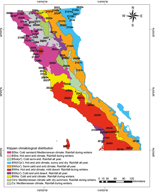
Fig 1 Climatological distribution of Baja California, Mexico, according to the Köppen classification.
2.1 Spline interpolation method
The maps for average annual rainfall (Fig. 2a), average daily temperature (Fig. 2b), and altitude above sea level (Fig. 2c) were obtained through a spatial interpolation using the spline method based on the climatological information provided by each station. Among several methods that were considered, such as the inverse distancing weighing method, the kriging method, and the natural neighbor interpolation method, the spline interpolation method was selected as the best. The result, although not shown in this paper, proves that for this case, the spline method presents the smallest mean square error. The average annual rainfall (Fig. 2a) was obtained by calculating the average annual value of rainfall for each station, and then proceeding to a spatial interpolation. The average daily temperature map (Fig. 2b) and the altitude above sea level maps (Fig. 2c) were obtained in a similar way by interpolating their respective variables.
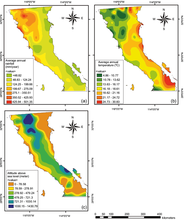
Fig. 2 Climatological and physiographic variables in Baja California. (a) Average annual rainfall (mm/yr). (b) Average annual temperature (ºC). (c) Altitude above sea level (m).
According to Hazenwinkel (2001), spline is a form of interpolation where the interpolator is a special type of polynomial called spline. This is very useful since the interpolation error can be smaller using this method. Also, this method is based on putting a curve through a determined number of points. The mathematical approach of this model is based on n + 1 nodes (x i , y i ) i = 0,1,…,n and interpolate between pairs of nodes (x i-1 , y i-1 ) and (x i , y i ) with polynomials y = q i (x), i = 1,2,…,n where the curvature of the curve
Y = f (x) (1)
Is:
 (2)
(2)
Therefore, the spline will minimize the bend, so y’ as well as y” will be continuous in the nodes:
 (3)
(3)
 (4)
(4)
for all values of i, 1 ≤ i ≤ n -1.
The next step is the fractal analysis of the data. To do so, 92 climatological stations with 30 yrs of daily rainfall data records were analyzed. In order to obtain the previously mentioned data, the Rapid Climatological Information Extractor (ERIC III) software and CLImate COMputing project (CLICOM), both of which include daily national climate data.
For the purpose of this research, the use of three different methods for calculating the Hurst exponent of each time series is required in order to get an average value that reflects a higher precision and reliability in the results. These three methods were the rescaled range analysis (R/S), the box counting method, and the multifractal detrended fluctuation analysis (MF-DFA) algorithm.
A determinant factor when selecting the method to apply was the number of available input parameters, meaning that the model would be more complex if it had a greater number of parameters. The considered methods in the present study are easy to apply and have been widely referenced in the recent literature (López-Lambraño et al., 2017). Also, the methods we applied allow detecting non-periodic cycles and long term correlations in random processes; furthermore, they are not influenced by the occurrence of probable lineal tendencies presented in series, and they manage to detect long-range correlations in non-stationary time series just as the MF-DFA does.
By employing the Benoit software, Hurst exponent values were obtained for both the R/S and the box counting methods. The computational algorithm for MF-DFA was programmed following the considerations established by Movahed et al. (2006).
2.2 Rescaled range method (R/S)
An alternative approach to the correlation quantification in a time series analysis was developed by Hurst (1951, 1956), who spent his entire life studying the hydrology of the Nile river, particularly on droughts and floods. Hurst considered the river’s flow as a time series and determined storage limits. Based on his studies, he empirically introduced the concept of R/S. Considering a time series, the summation of time series relative to their average value is:
 (5)
(5)
where the range is defined by
 (6)
(6)
with
 (7)
(7)
where  and σN are the mean and standard deviations of all the N values in the time series yn. From the previous equations, a value (RN/SN) is obtained for the time series yn. We substitute ᴛ by N in equations 5 to 7. The Hurst exponent (Hu), is obtained as:
 (8)
(8)
The rescaled range R/S (w) is defined as:
 (9)
(9)
where w is the window width and the symbols  represent the average values of a number of values of R(w). The foundation of the method is that, based on the self-affinity, it can be expected that
 (10)
(10)
In practice, for a determined value of w, a time series is subdivided by a number of intervals of width w, then R(w) and S(w) are calculated for each one, and R/S(w) as the average ratio R(w)/S(w). This procedure is repeated for a determined number of window widths, and the logarithms of R/S(w) are plotted against the logarithms of w. If the set has self-affinity, then the plot will follow a straight line whose slope is equal to the Hurst exponent H u . The fractal dimension of the set can be calculated from the Hurst exponent-fractal dimension relation:
 (11)
(11)
where D rs denotes the fractal dimension calculated by the rescaled range method.
2.3 Box counting method
According to Peñate et. al. (2013), the box counting method is based on dividing the space of observation (the time interval T) into n non-overlapping segments of characteristic size s, so that s = T/n for n = 2,3,4,…, and computing the number N(s) of intervals of length s occupied by events. If the distribution of events has a fractal structure, then the relationship N(s) = Cs D prevails. The fractal or box counting dimension D f is estimated from the slope D of the regression line of log(N(s)) on log(s). This parameter D f = |D| describes the strength of the events and can measure the phenomenon’s nature, since it quantifies the scale-invariant clustering of the time series. Clustering increases when D approaches 0. Hence, the smallest fractal dimensions correspond to clusters formed by events that occur sparsely. If D is close to 1, the events are randomly spaced in time. To sum up, the box counting method uses boxes to cover an object in order to find the fractal dimension. The signal is partitioned into boxes of various sizes and the amount of non-empty squares is counted. A log-log plot of the number of boxes vs. the size of the boxes is done. The box dimension is defined by the exponent D b in the relation
 (12)
(12)
where N(s) is the number of boxes with linear size s needed to cover the set of points distributed on a bidimensional plane. A number of boxes, proportional to a 1/s, are needed to cover the set of points on a line; proportional to 1/s 2 , to cover a set of points on a plane, etc.
In theory, for each box size, the grid should be configured in such a way that the minimum number of boxes is occupied. This can be achieved by rotating the grid for each box size in 90º and plotting the minimum value of N(d).
2.4 Multifractal detrended fluctuation analysis
According to Yuval and Broday (2010), Movahed et al. (2006) and Kantelhardt et al. (2002), the modified multifractal DFA (MF-DFA) procedure consists of five steps. Suppose that x k is a series of length N, and that this series is of compact support, i.e., x k = 0, only for an insignificant fraction of the values.
Step 1. Determination of the profile:
 (13)
(13)
Subtraction of the mean  is not compulsory, since it would be eliminated by the later detrending in the third step.
Step 2. Division of the profile Y(i) into N s = int(N/s) non-overlapping segments of equal lengths s. Since the length N of the series is often not a multiple of the considered timescale s, a short part at the end of the profile may remain. In order to disregard this part of the series, the same procedure is repeated starting from the opposite end. Thereby, 2N s segments are obtained altogether.
Step 3. Calculation of the local trend for each of the 2N s segments by a least square fit of the series. Then the variance should be determined:
 (14)
(14)
for each segment v, v = 1,…, N s , and:
 (15)
(15)
for v = N s + 1,…,2N s . Here y v (i) is the fitting polynomial in segment v. Linear, quadratic, cubic or higher order polynomials can be used in the fitting procedure. Since the detrending of the time series is done by the subtraction of the polynomial fits from the profile, different order DFA differ in their capability of eliminating trends in the series.
Step 4. Average over all segments to obtain the qth-order fluctuation function, defined as
 (16)
(16)
where, in general, the index variable q can take any real value except zero. For q = 2, the standard DFA procedure is retrieved. Generally, we are interested in how the generalized q-dependent fluctuation functions F q (s) depend on timescale s for different values of q. Hence, we must repeat steps 2, 3 and 4 for several timescales s. It is apparent that F q (s) will increase while s increases. Of course F q (s) depends on the DFA order m. By construction, F q (s) is only defined for s ≥ m + 2.
Step 5. Determination of the scaling behavior of the fluctuation functions by analyzing log-log plots of F q (s) versus s for each value of q. If the series x i are correlated by the long-range power-law, F q (s) increases, for large values of s, as a power law:
 (17)
(17)
In general, the exponent h(q) may depend on q. The exponent h(2) is identical to the well-known Hurst exponent (H u ).
A decimal fraction—as fractal dimension—allows describing fractal geometry as well as the heterogeneity of irregular sets, which enables us to record any lost data if traditional geometry representations were applied. A relationship between the fractal dimension and the Hurst coefficient for the used fractal methods is defined by 2H + 1 = 5 - 2D rs . If we solve the equation for D rs we obtain Eq, (11). This idea establishes a robust analysis, since long-term persistence conditions can be assessed, non-periodic cycles can be detected, and long-term random processes can be established. When we encounter a fractal dimension which is close to the unit, we can confirm highly persistent series and a limited variation.
2.5 Fractal considerations
In order to estimate the Hurst exponent for the proposed time series, the following considerations and time scales were taken into account:
1. Hurst exponent values calculated from the analysis of the complete time series. In order to estimate the H u value for this first consideration, the three methods were employed. Then the three obtained values were averaged.
2. Hurst exponent values calculated from the analysis of a time series in periods of 25 yrs. In this matter we followed the same procedure mentioned above. However, the time series was partitioned into two periods of 25 yrs.
3. Hurst exponent values calculated from the analysis of a time series in periods of 10 yrs.
4. Hurst exponent values calculated from the analysis of a time series in periods of 5 yrs. For considerations three and four, the procedure was done using the approach proposed in point two.
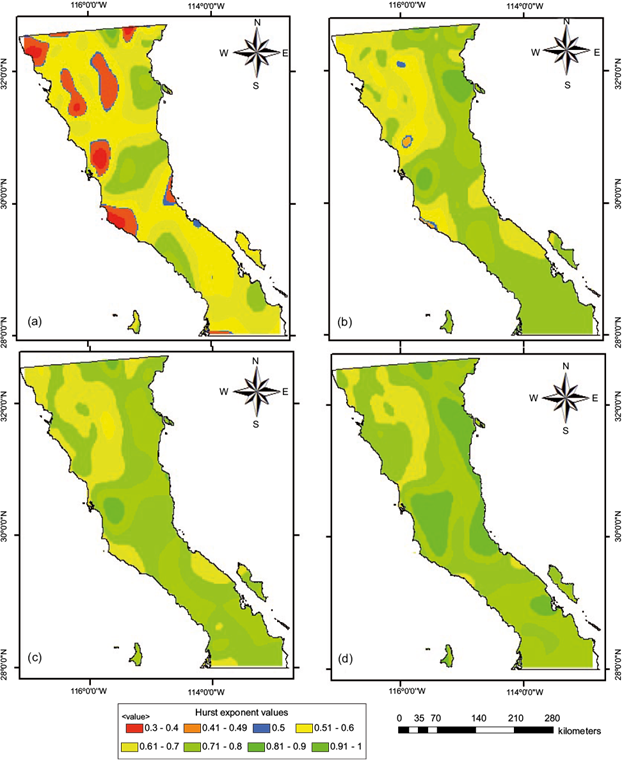
5. After obtaining the Hurst exponents from the climate stations, a spline interpolation was conducted; additionally, spatial distribution maps (presented below) were generated where the Hurst exponent values were interpolated based on the average results for each climate station. The maps for the complete time series (Fig. 3a) and for the time scales of 25 (Fig. 3b), 10 (Fig. 3c), and 5 yrs (Fig. 3d) were generated.
3. Results and discussion
Maps for Koppen’s climatological classification (Fig. 1), annual pluvial regime (Fig. 2a), average annual temperature (Fig. 2b) and meters above sea level (Fig. 2c) were generated from the data obtained from the 92 climate stations with more than 30 yrs of daily rainfall records (Tables I and II).
Table I Average Hurst exponent results for climatological stations in Baja California sorted by type of climate
| No. | Climatological station | Köppen climate classification | Latitude | Longitude | Average Hurst exponent for daily rainfall events (complete time series) |
| 2001 | Agua Caliente | BSks climate: cold semiarid Mediterranean. Rainfall during winters | 32.107 | -116.454 | 0.51 |
| 2003 | Bataquez | 32.551 | -115.069 | 0.61 | |
| 2005 | Boquilla de Santa Rosa l | 32.022 | -116.777 | 0.54 | |
| 2008 | Colonia Guerrero | 30.717 | -115.983 | 0.53 | |
| 2024 | El Testerazo | 32.296 | -116.534 | 0.65 | |
| 2029 | La Providencia | 30.969 | -116.157 | 0.57 | |
| 2035 | Ojos Negros | 31.912 | -116.265 | 0.5 | |
| 2036 | Olivares Mexicanos | 32.049 | -116.681 | 0.53 | |
| 2038 | Presa Rodríguez | 32.447 | -116.908 | 0.45 | |
| 2055 | San Telmo | 30.95 | -116.1 | 0.55 | |
| 2056 | San Vicente | 31.329 | -116.248 | 0.48 | |
| 2060 | Santa Cruz | 30.879 | -115.628 | 0.52 | |
| 2064 | Santo Domingo | 31.633 | -116.377 | 0.58 | |
| 2068 | Tijuana | 32.525 | -117.042 | 0.49 | |
| 2069 | Valle de las Palmas | 32.37 | -116.654 | 0.48 | |
| 2071 | Colonia valle de la trinidad | 31.356 | -115.696 | 0.51 | |
| 2079 | El Alamar | 31.836 | -116.204 | 0.54 | |
| 2089 | Ejido Emilio López Zamora | 31.104 | -116.168 | 0.68 | |
| 2091 | Ejido Ignacio López Ray | 31.288 | -116.264 | 0.55 | |
| 2092 | Ejido San Matías | 31.331 | -115.544 | 0.56 | |
| 2096 | La Calentura | 31.27 | -116.037 | 0.59 | |
| 2104 | El Ciprés | 31.79 | -116.588 | 0.59 | |
| 2106 | Maneadero | 31.696 | -116.573 | 0.57 | |
| 2108 | Punta Banda | 31.714 | -116.666 | 0.59 | |
| 2110 | Guayaquil | 29.967 | -115.097 | 0.65 | |
| 2118 | Valle San Rafael | 31.919 | -116.234 | 0.54 | |
| 2121 | El Hongo | 32.516 | -116.303 | 0.52 | |
| 2124 | El Carrizo II | 32.491 | -116.684 | 0.53 | |
| 2152 | Ejido J. Maria del Pino | 32.373 | -116.068 | 0.62 | |
| 2153 | Ejido Uruapan | 31.619 | -116.455 | 0.61 | |
| 2012 | Ejido J. María Morelos | BWk(x’) climate: cold arid desert. Rainfall all year | 28.3 | -114.026 | 0.65 |
| 2109 | Santa Rosalita | 28.668 | -114.237 | 0.69 | |
| 2009 | Colonia Juárez | BW(h’)(x’) climate: hot and arid, sunny and dry. Rainfall all year | 32.299 | -115.016 | 0.61 |
| 2011 | Delta | 32.353 | -115.189 | 0.65 | |
| 2016 | El barril | 28.302 | -112.878 | 0.61 | |
| 2020 | El mayor | 32.127 | -115.278 | 0.69 | |
| 2033 | Mexicali (dge) | 32.663 | -115.468 | 0.57 | |
| 2034 | Mexicali (smn) | 32.55 | -115.467 | 0.6 | |
| 2037 | Presa Morelos | 32.715 | -114.729 | 0.61 | |
| 2046 | San Felipe | 31.028 | -114.835 | 0.66 | |
| 2107 | Percebú | 30.886 | -114.779 | 0.78 | |
| 2139 | Colonia Rodríguez | 32.419 | -115.036 | 0.73 | |
| 2140 | Colonia Zaragoza | 32.61 | -115.531 | 0.86 | |
| 2141 | Compuerta Benassini | 32.57 | -115.111 | 0.63 | |
| 2145 | Rancho Williams | 32.624 | -114.878 | 0.61 | |
| 2154 | Colonia zacatecas | 32.06 | -115.059 | 0.71 | |
| 2002 | Bahía de los Ángeles | BWh(x’) climate: semicalid and arid. Rainfall all year | 28.604 | -113.556 | 0.65 |
| 2006 | Chapala | 29.488 | -114.364 | 0.57 | |
| 2059 | Santa Clara | 31.081 | -115.286 | 0.58 | |
| 2061 | Santa Gertrudis | 28.075 | -113.092 | 0.62 | |
| 2072 | Presa Emilio López Zamora | 31.896 | -115.597 | 0.47 | |
| 2093 | Ejido Valle de la Trinidad | 32.356 | -115.749 | 0.57 | |
| 2099 | Rancho los Algodones | 30.781 | -115.175 | 0.74 | |
| 2101 | El Centinela | 32.575 | -115.742 | 0.81 | |
| 2102 | La Ventana | 31.44 | -115.054 | 0.71 | |
| 2137 | Colonia Mariana | 32.259 | -115.322 | 0.65 | |
| 2146 | Colonia San Pedro Mártir | 31.038 | -115.204 | 0.6 | |
| 2151 | Agua de Chale | 30.638 | -114.75 | 0.68 | |
| 2023 | El Socorro | BWks climate: cold and arid. Rainfall during winters | 30.321 | -115.821 | 0.59 |
| 2031 | La Rumorosa | 32.549 | -116.046 | 0.6 | |
| 2032 | Las Escobas | 30.579 | -115.938 | 0.51 | |
| 2043 | San Agustín | 29.938 | -114.967 | 0.57 | |
| 2063 | Santa María del Mar | 30.402 | -115.888 | 0.54 | |
| 2086 | Ejido Jacume | 32.591 | -116.192 | 0.58 | |
| 2111 | Ejido Nueva Baja California | 30.517 | -115.931 | 0.62 | |
| 2015 | El Arco | BWhs climate: hot and arid, semicalid. Rainfall during winters | 28.029 | -113.396 | 0.59 |
| 2022 | El Rosario | 30.059 | -115.723 | 0.59 | |
| 2027 | Isla Cedros | 28.135 | -115.175 | 0.71 | |
| 2039 | Punta Prieta | 29.158 | -114.146 | 0.57 | |
| 2040 | Rancho Alegre | 28.229 | -113.755 | 0.59 | |
| 2041 | Nuevo Rosarito | 28.634 | -114.017 | 0.58 | |
| 2044 | San Borja | 28.735 | -113.753 | 0.57 | |
| 2051 | San Luis Baja California | 29.727 | -114.711 | 0.62 | |
| 2053 | San Miguel | 28.583 | -113.95 | 0.62 | |
| 2058 | Santa Catarina Sur | 29.722 | -115.13 | 0.54 | |
| 2084 | El Progreso | 29.968 | -115.191 | 0.6 | |
| 2085 | San Regis | 28.597 | -113.755 | 0.59 | |
| 2120 | Ejido México | 31.072 | -116.206 | 0.64 | |
| 2144 | Ensenada Blanca | 28.411 | -113.864 | 0.69 | |
| 2004 | Ignacio Zaragoza | Cs climate: Mediterranean. Rainfall during winters | 32.195 | -116.486 | 0.54 |
| 2014 | El Álamo | 31.593 | -116.054 | 0.52 | |
| 2019 | El Compadre | 32.338 | -116.254 | 0.58 | |
| 2021 | El Pinal | 32.183 | -116.292 | 0.55 | |
| 2045 | San Carlos | 31.785 | -116.464 | 0.55 | |
| 2049 | San Juan de Dios del Norte | 32.132 | -116.165 | 0.52 | |
| 2057 | Santa Catarina Norte | 31.657 | -115.824 | 0.51 | |
| 2065 | Santo Tomás | 31.792 | -116.406 | 0.47 | |
| 2088 | Ejido Heroes de la Independencia | 31.61 | -115.938 | 0.61 | |
| 2114 | Ejido Carmen Serdán | 32.244 | -116.584 | 0.62 | |
| 2050 | San Juan de Dios del Sur | BSok(x’) climate: cold semiarid. Rainfall all year | 30.184 | -115.137 | 0.69 |
Table II Averaged Hurst exponent results for climatological stations in Baja California for all time scales for daily rainfall events
| No. | Climatological station | Elevation (masl) | Average annual rainfall (mm yr-1) | Average annual temperature (ºC) | Average Hurst exponent for the different time scales | |||
| Complete time series | 25 yrs | 10 yrs | 5 yrs | |||||
| 2001 | Agua Caliente | 400 | 272.76 | 12.68 | 0.51 | 0.6 | 0.66 | 0.68 |
| 2002 | Bahía de los Ángeles | 4 | 67.31 | 21.98 | 0.65 | 0.74 | 0.79 | 0.81 |
| 2003 | Bataquez | 23 | 72.49 | 20.02 | 0.61 | 0.74 | 0.78 | 0.82 |
| 2004 | Ignacio Zaragoza | 540 | 297.63 | 12.21 | 0.54 | 0.62 | 0.69 | 0.73 |
| 2005 | Boquilla Santa Rosa de L. | 250 | 264.70 | 13.22 | 0.54 | 0.64 | 0.64 | 0.65 |
| 2006 | Chapala | 660 | 115.16 | 19.59 | 0.57 | 0.7 | 0.71 | 0.75 |
| 2008 | Colonia Guerrero | 30 | 159.04 | 15.34 | 0.53 | 0.61 | 0.67 | 0.71 |
| 2009 | Colonia Juárez | 17 | 59.73 | 19.01 | 0.61 | 0.68 | 0.78 | 0.79 |
| 2011 | Delta | 12 | 46.58 | 19.76 | 0.65 | 0.72 | 0.77 | 0.8 |
| 2012 | Ejido J. María Morelos | 20 | 62.74 | 15.53 | 0.65 | 0.77 | 0.79 | 0.85 |
| 2014 | El Álamo | 1115 | 268.82 | 13.66 | 0.52 | 0.6 | 0.66 | 0.72 |
| 2015 | El Arco | 288 | 102.75 | 17.62 | 0.59 | 0.74 | 0.78 | 0.86 |
| 2016 | El Barril | 50 | 81.31 | 24.12 | 0.61 | 0.76 | 0.78 | 0.85 |
| 2019 | El Compadre | 1110 | 308.55 | 18.84 | 0.58 | 0.68 | 0.63 | 0.69 |
| 2020 | El Mayor | 15 | 56.16 | 17.74 | 0.69 | 0.8 | 0.83 | 0.89 |
| 2021 | El Pinal | 1320 | 453.80 | 9.22 | 0.55 | 0.78 | 0.64 | 0.7 |
| 2022 | El Rosario | 40 | 168.59 | 16.78 | 0.59 | 0.72 | 0.76 | 0.81 |
| 2023 | El Socorro | 26 | 106.09 | 17.11 | 0.59 | 0.79 | 0.8 | 0.84 |
| 2024 | El Testerazo | 380 | 240.58 | 11.72 | 0.65 | 0.72 | 0.76 | 0.76 |
| 2027 | Isla Cedros | 3 | 62.73 | 19.74 | 0.71 | 0.81 | 0.84 | 0.87 |
| 2029 | La Providencia | 40 | 257.25 | 13.93 | 0.57 | 0.72 | 0.73 | 0.78 |
| 2031 | La Rumorosa | 1232 | 135.59 | 14.7 | 0.6 | 0.73 | 0.73 | 0.79 |
| 2032 | Las Escobas | 30 | 134.61 | 15.03 | 0.51 | 0.7 | 0.75 | 0.8 |
| 2033 | Mexicali (DGE) | 3 | 73.93 | 18.8 | 0.57 | 0.76 | 0.75 | 0.81 |
| 2034 | Mexicali (SMN) | 3 | 73.54 | 20.24 | 0.6 | 0.72 | 0.77 | 0.88 |
| 2035 | Ojos Negros | 680 | 226.76 | 12.73 | 0.5 | 0.61 | 0.66 | 0.69 |
| 2036 | Olivares Mexicanos | 340 | 279.97 | 14.46 | 0.53 | 0.68 | 0.7 | 0.76 |
| 2037 | Presa Morelos | 40 | 62.43 | 17.83 | 0.61 | 0.66 | 0.74 | 0.82 |
| 2038 | Presa Rodríguez | 120 | 232.25 | 14.63 | 0.45 | 0.62 | 0.65 | 0.7 |
| 2039 | Punta Prieta | 325 | 89.93 | 16.47 | 0.57 | 0.74 | 0.76 | 0.84 |
| 2040 | Rancho Alegre | 120 | 120.32 | 15.83 | 0.59 | 0.75 | 0.75 | 0.82 |
| 2041 | Nuevo Rosarito | 20 | 110.30 | 16.84 | 0.58 | 0.75 | 0.74 | 0.79 |
| 2043 | San Agustín | 552 | 111.09 | 17.13 | 0.57 | 0.75 | 0.76 | 0.81 |
| 2044 | San Borja | 445 | 104.99 | 18.03 | 0.57 | 0.73 | 0.76 | 0.85 |
| 2045 | San Carlos | 164 | 263.38 | 15.19 | 0.55 | 0.68 | 0.69 | 0.75 |
| 2046 | San Felipe | 10 | 64.96 | 22.5 | 0.66 | 0.84 | 0.86 | 0.94 |
| 2049 | San Juan de Dios del Norte | 1280 | 362.93 | 12.09 | 0.52 | 0.58 | 0.61 | 0.65 |
| 2050 | San Juan de Dios del Sur | 600 | 120.74 | 16.7 | 0.69 | 0.73 | 0.76 | 0.8 |
| 2051 | San Luis Baja California | 480 | 92.75 | 17.82 | 0.62 | 0.81 | 0.83 | 0.89 |
| 2053 | San Miguel | 440 | 124.93 | 19.44 | 0.62 | 0.71 | 0.7 | 0.77 |
| 2055 | San Telmo | 60 | 192.05 | 13.8 | 0.55 | 0.65 | 0.73 | 0.76 |
| 2056 | San Vicente | 110 | 211.76 | 13.21 | 0.48 | 0.65 | 0.73 | 0.74 |
| 2057 | Santa Catarina Norte | 1150 | 248.74 | 14.53 | 0.51 | 0.6 | 0.62 | 0.66 |
| 2058 | Santa Catarina Sur | 317 | 137.61 | 16.38 | 0.54 | 0.71 | 0.73 | 0.79 |
| 2059 | Santa Clara | 410 | 128.24 | 18.84 | 0.58 | 0.69 | 0.73 | 0.8 |
| 2060 | Santa Cruz | 980 | 265.14 | 15.57 | 0.52 | 0.63 | 0.66 | 0.71 |
| 2061 | Santa Gertrudis | 400 | 105.45 | 18.06 | 0.62 | 0.72 | 0.75 | 0.84 |
| 2063 | Santa María del Mar | 28 | 160.65 | 14.95 | 0.54 | 0.71 | 0.73 | 0.79 |
| 2064 | Santo Domingo | 250 | 211.54 | 14.06 | 0.58 | 0.72 | 0.74 | 0.79 |
| 2065 | Santo Tomás | 180 | 262.63 | 16.43 | 0.47 | 0.62 | 0.65 | 0.67 |
| 2068 | Tijuana | 20 | 220.40 | 15.22 | 0.49 | 0.62 | 0.66 | 0.72 |
| 2069 | Valle de las Palmas | 280 | 206.94 | 12.74 | 0.48 | 0.63 | 0.69 | 0.72 |
| 2071 | Colonia Valle de la Trinidad | 740 | 204.73 | 10.59 | 0.51 | 0.59 | 0.62 | 0.67 |
| 2072 | Presa Emilio López Zamora | 43 | 248.41 | 14.58 | 0.47 | 0.64 | 0.66 | 0.69 |
| 2079 | El Alamar | 710 | 264.09 | 12.8 | 0.54 | 0.63 | 0.68 | 0.69 |
| 2084 | El Progreso | 517 | 135.61 | 17.64 | 0.6 | 0.73 | 0.76 | 0.83 |
| 2085 | San Regis | 495 | 132.94 | 17.97 | 0.59 | 0.73 | 0.73 | 0.78 |
| 2086 | Ejido Jacume | 860 | 214.49 | 13.24 | 0.58 | 0.67 | 0.72 | 0.74 |
| 2088 | Ejido Héroes de la Independencia | 1000 | 263.63 | 14.08 | 0.61 | 0.71 | 0.72 | 0.75 |
| 2089 | Ejido Emilio López Zamora | 180 | 187.23 | 14 | 0.68 | 0.75 | 0.75 | 0.78 |
| 2091 | Ejido Ignacio López Ray | 170 | 269.95 | 11.88 | 0.55 | 0.67 | 0.69 | 0.74 |
| 2092 | Ejido San Matías | 968 | 214.29 | 15.95 | 0.56 | 0.63 | 0.67 | 0.73 |
| 2093 | Ejido Valle de la Trinidad | 780 | 231.19 | 11.6 | 0.57 | 0.71 | 0.74 | 0.79 |
| 2096 | La Calentura | 210 | 209.38 | 14.27 | 0.59 | 0.69 | 0.72 | 0.77 |
| 2099 | Rancho los Algodones | 460 | 72.87 | 19.22 | 0.74 | 0.78 | 0.8 | 0.87 |
| 2101 | El Centinela | 50 | 46.13 | 20.7 | 0.81 | 0.9 | 0.88 | 0.93 |
| 2102 | La Ventana | 16 | 36.33 | 21.3 | 0.71 | 0.88 | 0.88 | 0.92 |
| 2104 | El Ciprés | 8 | 202.84 | 15.25 | 0.59 | 0.7 | 0.72 | 0.74 |
| 2106 | Maneadero | 50 | 202.03 | 15.28 | 0.57 | 0.69 | 0.73 | 0.73 |
| 2107 | Percebú | 4 | 44.09 | 19.12 | 0.78 | 0.87 | 0.9 | 0.92 |
| 2108 | Punta Banda | 15 | 260.61 | 15.13 | 0.59 | 0.7 | 0.72 | 0.76 |
| 2109 | Santa Rosalita | 8 | 136.02 | 16.64 | 0.69 | 0.78 | 0.82 | 0.87 |
| 2110 | Guayaquil | 530 | 123.51 | 17 | 0.65 | 0.8 | 0.77 | 0.72 |
| 2111 | Ejido Nueva Baja California | 17 | 139.68 | 14.13 | 0.62 | 0.72 | 0.74 | 0.77 |
| 2114 | Ejido Carmen Serdán | 560 | 234.56 | 11.57 | 0.62 | 0.72 | 0.74 | 0.77 |
| 2118 | Valle San Rafael | 721 | 218.41 | 12.45 | 0.54 | 0.66 | 0.69 | 0.71 |
| 2120 | Ejido México | 75 | 176.97 | 13.61 | 0.64 | 0.71 | 0.75 | 0.78 |
| 2121 | El Hongo | 960 | 291.13 | 12.55 | 0.52 | 0.61 | 0.63 | 0.67 |
| 2124 | El Carrizo II | 300 | 233.74 | 13.59 | 0.53 | 0.63 | 0.65 | 0.68 |
| 2137 | Colonia Mariana | 9 | 57.61 | 19.4 | 0.65 | 0.78 | 0.75 | 0.82 |
| 2139 | Colonia Rodríguez | 17 | 36.84 | 18 | 0.73 | 0.88 | 0.82 | 0.9 |
| 2140 | Colonia Zaragoza | 8 | 65.17 | 12.43 | 0.86 | 0.82 | 0.88 | 0.94 |
| 2141 | Compuerta Benassini | 20 | 55.11 | 17.9 | 0.63 | 0.8 | 0.75 | 0.84 |
| 2144 | Ensenada Blanca | 10 | 89.08 | 19.7 | 0.69 | 0.75 | 0.82 | 0.84 |
| 2145 | Rancho Williams | 29 | 63.06 | 20.57 | 0.61 | 0.77 | 0.73 | 0.83 |
| 2146 | Colonia San Pedro Mártir | 416 | 106.32 | 16.19 | 0.6 | 0.75 | 0.74 | 0.81 |
| 2151 | Agua de Chale | 5 | 53.13 | 22.59 | 0.68 | 0.83 | 0.82 | 0.88 |
| 2152 | Ejido J. María del Pino | 1380 | 273.63 | 8.7 | 0.62 | 0.74 | 0.72 | 0.75 |
| 2153 | Ejido Uruapan | 195 | 288.55 | 13.9 | 0.61 | 0.7 | 0.72 | 0.75 |
| 2154 | Colonia Zacatecas | 12 | 53.55 | 18.46 | 0.71 | 0.81 | 0.8 | 0.87 |
Considering the classification of climates in Baja California (Fig. 1), it can be seen that the values of the Hurst exponent (H u ) may be associated with the climatological conditions of the analyzed region, meaning that climates with daily rainfall regime during winter (BSKS, Cs, BWks and BWhs) obtain lower H u values (between 0.4 and 0.6), corresponding to persistent and anti-persistent behaviors. Compared to other studies, our results are similar to those obtained by Gutiérrez et al. (2006) in Australia, with BWhs climate and H u values between 0.4 and 0.56; however, they differ from the results obtained by Yuval and Broday (2010) in Israel with BWhs and Cs climates, and H u values of 0.7, as well as Zhou et al. (2005) in Botswana with climate BWhs and H u values from 0.55 to 0.92. For climates with daily rainfall regime throughout the year-BWk(x’), BW(h’)(x’), BWh(x’) and BSok(x’)- the obtained values are ranging between 0.57 and 0.86, meaning that there is a persistent behavior which is similar to the result obtained by Rehman (2009) in Saudi Arabia with BWh(x’) climate and H u values between 0.59 and 0.71. Since climates with rainfall throughout the year are predominant in Baja California, most of the registered precipitation events show a persistent behavior over time. Climates that have very arid and semi-arid conditions with daily rainfall throughout the year BWh(x’) and climates with very arid and warm conditions with the same rainfall regime BW(h’)(x’) cover the state of Baja California from north to south, exhibiting a high variability in the H u value. The region comprising BWh(x’) and BW(h’)(x’) climates is delimited by the geographical coordinates 32.716º N, 114.719º W, and 29.943º N, 114.98º W, where the obtained H u values vary from 0.62 to 0.88, meaning there is a persistent behavior. Whereas, in the region limited by 29.943º N, 114.963º W, and 28.743º N, 113.745º W, H u values for the climates in consideration vary from 0.5 to 0.58, which indicates a tendency to random behavior. An anti-persistent behavior in the rainfall series can hinder the prediction of a new rainfall event. The time of the year that does not present meaningful rainfall events can be the responsible for the anti-persistent behavior in the series (Velásquez et al., 2013).
From Table II and Figure 2c, which shows the variation of altitudes in Baja California, it can be observed that the highest altitudes, corresponding to the Sierra Juárez and Sierra San Pedro Mártir, are located in the central area. Moreover, comparing this map with the maps for annual precipitation (Fig. 2a) and average daily temperature (Fig. 2b), it is evident that regions in the studied area with higher altitudes have lower values for average daily temperatures, as well as greater values for average annual rainfall, in contrast with areas with altitudes close to the sea level. According to Table II, two climatological stations, Delta and San Vicente, are considered in order to illustrate the previously mentioned behavior. The Delta station is located at 12 masl, while the San Vicente station is located at 1150 masl. In Figure 2 it may be seen that the average annual rainfall regime is very low in Delta (46.65 mm yr-1) compared to San Vicente (248.7 mm yr-1). Regarding average daily temperature, the stations Delta and San Vicente reported 19.76 and 13.21 ºC, respectively.
It can be established that in Baja California, the average annual rainfall has a direct relation with the physiographic and altitude variables. The average annual temperature has a proportional inverse correlation with the magnitude of the average annual rainfall.
Given the importance of assessing the fractal behavior of the daily rainfall series and analyzing the variability of the H u at different time scales, an analysis was carried out considering the previously mentioned time scales, which correspond to H u values resulting from the analysis of the complete time series for rainfall daily events, as well as for the different time scales (25, 10, and 5 yrs).
Table II depicts the behavior of Hurst values for daily rainfall events at different time scales where reported. From the data analysis two main behavior patterns can be noticed for each of the time series regarding the analyzed variable: anti-persistent and persistent. Both of these behavior patterns will be discussed below.
According to Table II, the stations Presa Rodríguez, San Vicente, Tijuana, Valle de las Palmas, Presa Emilio López Zamora, and Santo Tomás, which are located in the northeast region of Baja California, presented the following H u values: 0.45, 0.48, 0.49, 0.48. 0.47 and 0.47, respectively, i.e., they are anti-persistent in time. This means that rainfall events that take place in this region have a high probability of showing a positive increasing behavior, followed by a decreasing behavior in its record values and vice versa. According to Malamud and Turcotte (1999), an anti-persistent time series will have a stationary behavior in time; due to the increases and decreases that compensate each other, statistical moments are independent from the time series. Rehman (2009) establishes that, in the case of rainfall, an anti-persistent behavior indicates a lesser dependency in accordance with previously stated values.
Nevertheless, when the rainfall series in the previously mentioned stations were analyzed in 25-yrs scales, the Hurst values were reported as follows: 0.62, 0.65, 0.62, 0.63, 0.64 and 0.62, respectively. These values indicate a persistent behavior in time, which means that if the rainfall series registers a positive increase, it is more likely that a positive increase will follow. This implies that each rainfall event has a degree of occurrence over future events or in its long-term behavioral memory.
From the analysis of the previously mentioned stations for 10- and 5-yr increases in the Hurst values, considering this are noticeable and show a persistent behavior through time, it can be found that the H u increases while establishing shorter time scales.
Anti-persistent series kept a positive increase tendency with minor negative increases; thus, while considering shorter periods of time (25, 10, 5 yrs), it is reasonable that series start to behave in a more persistent manner. This is due to the fact that the shorter the considered time scale, the greater the possibility to analyze a time period with a predominant behavior (which in in this case is persistent); this could explain the increase in the Hurst values in the analyzed rainfall series.
Continuing with the analysis of the remaining 86 stations, and considering the established time scales, increases in the Hurst values are noticeable with values greater than 0.5, indicating they keep a persistent behavior tendency. This means that rainfall series are not stationary and moments are dependent on the time scale. Persistency is an indicator that present events not only influence the near future but they will also have an impact in the long term.
A geospatialization of the H u values obtained at different time scales and reported on Table III, was carried out to allow the study of the spatial and temporal variability in Baja California (Fig. 3).
Table III Correlation matrix among geographic coordinates and fractal statistics.
| Longitude | Latitude | Altitude | D rs | H u | Average annual rainfall (mm yr-1) |
Median | SD | Temperature | |
| Longitude | 1 | -0.76 | -0.20 | -0.40 | 0.40 | -0.68 | -0.68 | -0.59 | 0.66 |
| Latitude | 1 | 0.15 | 0.11 | -0.11 | 0.32 | 0.34 | 0.21 | -0.35 | |
| Altitude | 1 | 0.31 | -0.31 | 0.60 | 0.59 | 0.55 | -0.47 | ||
| D rs | 1 | -1.00 | 0.62 | 0.66 | 0.46 | -0.43 | |||
| H u | 1 | -0.63 | -0.66 | -0.46 | 0.43 | ||||
| Average annual rainfall (mm yr-1) | 1 | 0.99 | 0.92 | -0.77 | |||||
| Median | 1 | 0.87 | -0.76 | ||||||
| SD | 1.0 | -0.75 | |||||||
| Temperature | 1 |
D rs : fractal dimension; H u : Hurst exponent; SD: standard deviation.
Three areas with different behavior regarding the H u can be noticed in Figure 3a: an anti-persistent area, a random area, and a persistent area. However, when a 25-yrs time scale is considered, the anti-persistent and indefinite areas start to decrease, as shown in Fig. 3b. Considering the 10- and 5-yrs time scales, a persistent behavior is noticeable throughout Baja California, as shown in Figure 3c, d.
Figure 3 shows a persistent tendency in the time series of the analyzed periods; however, we were able to identify a gradual increase in the H u when time series were segmented in periods. A possible explanation for this behavior is that non-segmented time series take into consideration all sudden changes expressed in terms of variable increase/decrease, which can influence the possible presence of anti-persistent behavior patterns. Nonetheless, when an analysis is carried out in segmented time series, there is a possibility that sudden changes cannot be noticed, which directly affects the persistence strength of the time series and causes a gradual increase in the H u values; however, fractality prevails in the series.
Temporal behavior of rainfall time series may be regionalized in space in order to study its relationship with geographical and physiographical variables. Figure 4a shows that the relationship between annual rainfall and the H u is fairly convincing (r = 0.63); also, according to the slope of the fitting line, this has an inverse relationship, and in Figure 4b, the H u of the time series is also moderately influenced by the annual temperature (r = 0.43). The altitude effect on the H u is weak (r = 0.31), which is shown in Figure 4c. It might be expected that the altitude effect on the dynamics of rainfall and temperature series would be especially strong. Actually, in Figure 4d the results show that there is a moderate relationship between temperature and altitude (r = -0.47) and in Figure 4e the annual rainfall also seems to be associated with altitude (r = 0.60). Another important parameter that determines the structural pattern in rainfall time series is the number of rainy days. In this research, we found a strong correlation (r = 0.81) between the number of rainy days and the H u (Fig. 4f); these results are similar to those found by Velásquez et al. (2013).
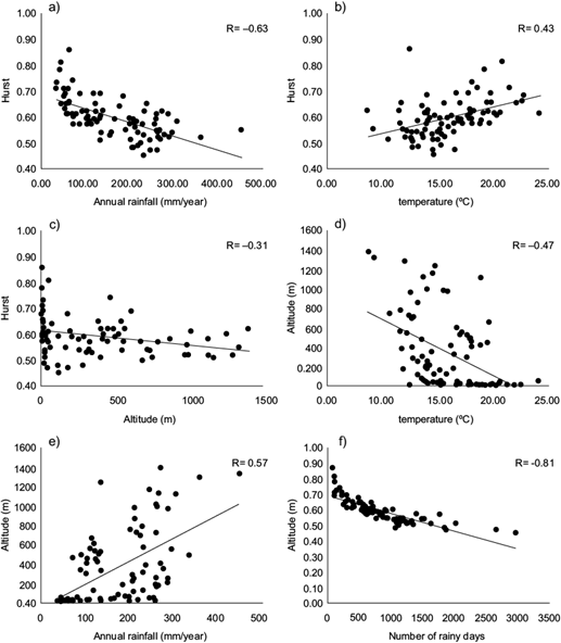
Fig. 4 Correlation analysis between the following variables: (a) H u (complete time series) and average annual rainfall; (b) H u (complete time series) and average annual temperature; (c) H u (complete time series) and altitude (Z); (d) altitude (Z) and average annual temperature; (e) Elevation (Z) and average annual rainfall; (f) H u and days of precipitation.
It should be noted that for the semiarid to arid conditions of Baja California, we established a correlation matrix among geographic coordinates and fractal statistics, which is shown in Table III. High correlations between fractal statistics mean a great interdependence, whereas these significant correlations between geographical coordinates and descriptive statistics suggest the strong influence of orography on rainfall (Magallanes et al. 2015), which is shown in Table III, where the relationship between H u values and longitude is a significant positive correlation (r = 0.40) and a significant negative correlation (r = -0.40) between the fractal dimension and longitude. The present findings strongly suggest that the D rs values of precipitation decrease as longitude increases, and H u increases as longitude does. The output tells us that a very weak relationship between Hurst exponent values and latitude is -0.11 for this data set. The relationship is negative. As latitude increases, the H u value rate decreases.
4. Conclusions
Even though three methods (MDFA, box counting, and R/S) were utilized to calculate the H u for each analyzed scale time, it is difficult to determine which of these methods is the most efficient; however, the R/S method has been reported as the most used one.
Registered daily rainfall series throughout Baja California can be characterized by using the H u , having as a result a tendency to present a persistent behavior. Thus, when a positive increase is registered, it is more likely that the following increase will be positive as well.
The Hurst exponents obtained from the rainfall time series are a measure to show a degree of dependency to the series, and can also explain the spatial and temporal behavior of rainfall in Baja California. This study suggests that rainfall series which took place in climates such as BWk(x’), BW(h’)(x’), BWh(x’), and BSok(x’), presented a persistent behavior in time, which is due to H u values fluctuating between 0.57 and 0.86. On the other hand, rainfall series which took place in climates such as BSks, Cs, BWks, and BWhs, showed a persistent and anti-persistent behavior, which is due to H u values ranging from 0.4 to 0.6.
The existence of a dependency between rainfall and temperature as climate variables in relation to altitude can be noticed. Regions with altitudes close to the sea level tend to register the highest temperature values, as well as the lowest average annual rainfall. It can be established that a proportional inverse relation between altitude and temperature exists, as well as a proportional direct relation between altitude and rainfall.
Taking into account the H u used in this research, a proportional inverse relation with altitude and rainfall can be noticed; in regions that are close to the sea level, high values can be reported; on the other hand, in regions where the average annual rainfall is high the analysis showed low values for the H u . It can be confirmed that the H u depends on the climatological conditions and physiographic characteristics of a specific region.
It can be found that the series persistency is stronger when shorter time scales (25, 10, 5 yrs in this research) are considered. The greater the number of time scales considered for analyzing rainfall series, the greater the possibility of understanding its behavior and tendencies.
By geospatializing the H u of the rainfall series, its variability regarding different climates in Baja California was traced and made visible. Besides, it provided data for the rainfall spatial-temporal behavior on this region.
Finally, it can be confirmed that fractal theory provides information that allows analyzing the occurrence of a climatological variable, such as rainfall (in the case of this research). This provides a useful tool to study and mitigate climate change in a given region.
It is recommended to use the multifractal theory in future researches, having as main purpose the opportunity to study the scale invariability from a mathematical perspective and to describe the climatic variable behavior with potential laws which are characterized by its exponents.
Multifractal theory allows describing precipitation behavior through potential laws that are characterized by their own exponents. It also constitutes a valid tool for the conceptualization of possible precipitation changes over time.

