2.1 Study domain

The study area covers Punjab, Haryana and Uttarakhand states, which are located in northern India. Punjab and Haryana are well-formed plains with elevation ranging from 200 to 800 m. They comprise the intensive agricultural zones of the country with urban parcels in growing phase after the late 1990s. Uttarakhand is located in the foothills of the Himalayan mountain ranges, having 86% of mountainous area, 65% of its territory being covered with forest land-use. The regions of interest receive most of the rainfall from the south-west monsoon covering the months of June to September.

2.2 Model description and setup

The WRF model (^{Skamarock et al., 2008}) version 3.4.1 (http://www.wrf-model.org) was used for forecasting weather parameters in this study. The mesoscale numerical model serves both for operational forecasting and regional atmospheric modelling. It is a limited-area, non-hydrostatic (with hydrostatic option) primitive equation model with multiple options for various physical parameterization schemes. Physics options used in this study include the ^{Kain-Fritsch cumulus parameterization scheme (Kain, 2004)} and the Purdue ^{Lin scheme (Lin et al., 1983)} for microphysics. The planetary boundary layer parameterizations are based on the Yonsei University boundary layer scheme (^{Hong et al., 2006}), and definition of the land surface process is based on the multi-layer Noah land surface model (LSM) model (^{Chen and Dudhia, 2001}). The long-wave radiation scheme is based on the Rapid Radiative Transfer Model (RRTM) (^{Mlawer et al., 1997}) and the Dudhia scheme (^{Dudhia, 1989}) represents short-wave radiation. The selected set of physics options has proven to give good results for the Indian domain (^{Ravindranath et al., 2010}; ^{Kumar et al., 2013}).

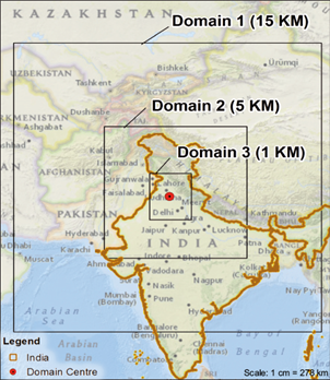
The setup contains three domains configured with one parent and two nests implemented with two-way nesting options. The three domains were run at 15, 5 and 1 km resolutions, respectively (Fig. 1). The centre point was fixed at 76º 14’ 13” E, 30º 18’ 8” N with the parent domain (15 km resolution) covering parts of Asia (225 × 270 grid points). The first nest (5 km resolution) has 325 × 375 grid points spanning to an extent covering northern parts of India. The second nest (1 km) roughly delimits the study area with 575 × 550 grid points and is the domain used for analysis. All the domains are terrain-following and have 36 vertical levels with the top of the atmosphere located at 50 hPa.

Fig. 1 Model domains. 

2.3 Simulation experiments

The control run represents a simulation by the WRF model with the default datasets, and the modified run is the simulation with updated datasets.

2.4 Model input data and analysis

2.4.1 Land surface datasets

The role of vegetation parameters in WRF is to estimate evapotranspiration components such as soil evaporation, wet canopy evaporation and canopy transpiration, and thus simulate surface energy balance in the Noah land surface model. Besides, land-use types also represent land surface parameters like albedo, roughness, emissivity and LAI within the model that are vital parameters, accounting for the energy partitioning at the surface. DEM is used in determining the displacement height and roughness length in the lower surface level, modulating the surface heat fluxes and the exchange coefficients within the planetary boundary layer (^{Chen and Dudhia, 2001}).

Most of the studies using meteorological models (MM5, Eta, REMO, RCM) including the WRF had been using coarser resolution data. For example, LULC at 1 km resolution based on the U.S. Geological Survey (USGS) land classification scheme derived from 1-yr (1992-1993 cycle) temporal AVHRR data (^{Loveland et al., 2000}). The USGS data lacks the finer details of land cover classes and presumably are outdated since significant changes in global land cover took place post-1993 (^{Ravindranath et al., 2010}). In this study, multi-temporal satellite datasets from the Advanced Wide Field Sensor (AWiFS) onboard the IRS-P6 satellite, is used to derive LULC maps based on supervised classification (2008-2009 cycle), which is also verified by ground truth procedures (^{Biswadip, 2014}). AWiFS has a spatial resolution of 58 m, and the land-use was prepared at a scale of about 1:250 000 under national repository programs of the Indian Space Research Organization (ISRO). AWiFS LULC captures the spatial variability of the cropping pattern using three land-use classes, viz. Kharif, Rabi and Zaid, representing the different crop seasons in India. The product also accurately represents other land-uses like forest types, urban, water bodies and wasteland. As concluded by ^{Sertel et al. (2009)}, the default land-use data is affected by outdated nature and misclassification of the land-use type due to the coarser resolution. In domains 2 and 3, which comprise the region of interest, both errors are prevalent. Land use changes are widespread in the Indo-Gangetic plains (Fig. 2a, b) aligned with the observations made by ^{Ravindranath et al. (2010)}. For example, about 22% of the area that was classified as dry cropland in the USGS dataset has been categorized as irrigated cropland in the AWiFS dataset, which is the reflection of technological advancements post 2000. The increase in barren lands due to land degradation in the neighborhood of the Thar Desert, Rajasthan, has led to extended desertification, which is captured well in the updated LULC dataset. Urban areas surrounding Delhi, as well as in Punjab and Haryana states have drastically increased since the 1990s (^{Rahman et al., 2011}); accordingly, 7% of irrigated cropland and 2% of shrubland category in the default data belongs to urban land-use in the modified dataset. Snow cover over the northern part of Jammu and Kashmir has increased marginally, while the barren lands have declined significantly. Misrepresentations are prominent in the forest regions where 5 and 3% of evergreen forest (actual land-use) appear as deciduous forest and shrubland categories in the default dataset. Similarly, about 2% of the deciduous forest was represented as cropland in the default dataset. Thus, an overall change of about 40% is observed within the study area, which makes the modified dataset very pertinent to the study. The modification captures the spatiotemporal variability of the dynamic land-use types in the region of interest. Figure 3 exemplifies a prominent case in the Uttarakhand region, where the better representation of the land-use variability in Shivalik and adjacent areas by the modified dataset is evident.

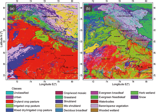
Fig. 2 Dominant land use/land cover categories. (a) Default (USGS) land cover data. (b) Modified (AWiFS) land cover data. 

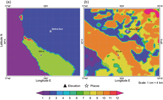
Fig. 3 Comparison between land use and land cover represented at model’s resolution (1 km). (a) Default (USGS). (b) AWiFS data modified input. 

The terrain is represented with the latest 90 m resolution DEM from the SRTM, a joint NASA-NGA partnership, available from http://srtm.csi.cgiar.org. The accuracy of the generated DEM is high, which is validated across the globe. The distinct differences are exhibited in areas with complex terrain, while in plains contrasts are marginal. For example, Figure 4 represents the variation in the elevation of Uttarakhand state captured well by the SRTM dataset. The default coarser resolution DEM showed a gradual increase in elevation, while the modified DEM captures the variability in elevation, particularly over the Shivalik ranges (lower Himalayan regions), the valley in between (Dehradun and adjacent areas), and the increasing elevation towards the upper Himalayas, which is not prominent in the former.

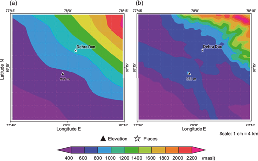
Fig. 4 Complexity of the terrain (m) captured at models’ resolution (1 km). (a) Default (DEM [GTOPO 30]). (b) DEM (SRTM) modified input. The units are in meters above mean sea level. 

LAI is defined as a one-sided green leaf area per unit ground area. Conceptually it is a representation of the amount of ground covered or left uncovered. The model typically uses a default lookup table (LUT) approach in which a constant LAI is assigned to each USGS land-use category. Such static LAI for each land cover category at model’s resolution often fails to capture the spatial and temporal heterogeneity of the index, which is the vertical component of the vegetation. LAI is essential to address the partitioning of energy between latent and sensible flux components. Prescription of spatially and temporally explicit information on LAI to the WRF model is thus inevitable (^{Tian et al., 2004}). Model initialization is done with a freely available and globally validated MODIS-LAI product (^{Pandya et al., 2003}; ^{Yuan et al., 2011}). The eight-day composite LAI product at 1-km resolution is obtained from https://lpdaac.usgs.gov, a website maintained by the NASA Land Processes Distributed Active Archive Center (LP-DAAC), which is processed to get monthly LAI datasets. Significant dissimilarities are observed throughout the study domain, revealing that the new LAI information from MODIS has better captured the spatial and temporal variability of LAI within individual vegetation land-use types. On the contrary, LAI based on the LUT approach yielded unrealistic values. For instance, LAI values are in the range of 4-5 for the deciduous forest in Shivalik hills, which is a rarity at the beginning of the winter season due to shedding of leaves. In another instance, modified dataset correctly captured low LAI values occurring in the agricultural lands of Punjab due to maturity/harvest of crops during October, while the default LUT approach showed LAI values in the range of 3.5-4, which is considerably high in that month (Fig. 5).

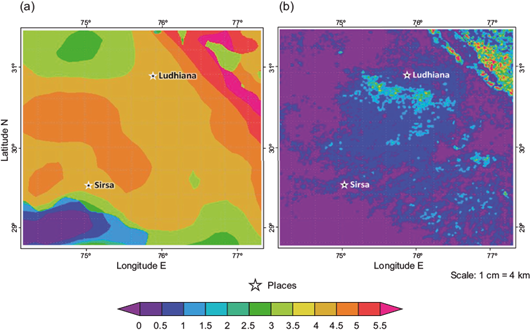
Fig. 5 Representation of LAI (m2 m-2) between the two sources at model’s resolution (1 km). (a) Default ( LUT-USGS land use classes). (b) MODIS LAI (modified input). 

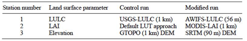
The different land surface datasets used for the simulations are tabulated in Table I. Upscaling from finer resolution to coarser resolution is always superior to direct usage of the coarser dataset, which is addressed in this study. Even if the model is implemented in coarser resolutions, an external upscaling of the modified input like the one explained below is necessary to avoid interpolation uncertainties being introduced within the model. Smoothening of the finer resolution images (to avoid noise) are performed externally, and the smoothened dataset is upscaled to the model’s resolution (here, 1 km) using the nearest neighbor method, before feeding input into the model. ^{Walker and Leone (1994)} demonstrated the importance of smoothening, especially for DEM. Figures 3, 4 and 5 represent the high variability at model’s resolution, thus proving the need for external smoothening and interpolation to retain essential classes/values.

Table I Land surface inputs for the control and modified runs of the WRF. 

2.5. Evaluation methods

The performance of the WRF model for different cases is evaluated with the data of 15 automatic weather stations (AWS) installed by the Indian Space Research Organization (ISRO) within Punjab and Haryana (Fig. 6a). The bilinear interpolation method is used to select the pixel from the model’s output that is closest to the observational station. Temperature and humidity are considered at a 2 m height while wind speed is considered at a 10 m height for verification.

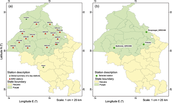
Fig. 6 Meteorological stations network. (a) Stations within the area of interest. (b) Selected meteorological stations for validation. 

Statistical measures such as mean bias, root mean square error (RMSE) and mean absolute percent error (MAPE) are used to evaluate the performance of the WRF model’s forecast. RMSE serves to aggregate the magnitudes of errors in predictions for various times into a single measure of predictive power, and is a good measure to compare forecasting errors of different models for a particular variable. MAPE essentially combines the individual percentage errors without offsetting the negative and positive values.

The improvement factor, which is found to be very relevant to compare the performance of climate models/simulations (^{Kumar et al., 2013}), is used to compare the performance of the control and modified runs. It provides the percentage improvement of one simulation (here, modified run) over the other (default run), and is given by:

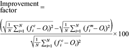(1)

where f _i ^c is the forecast of the control run (WRF-CNT) at the ith observation, f _i ^m is the forecast of the modified run (WRF-EXT) at the ith observation, and O _i is the actual observed data at the ith observation.

Individual sensitivity analyses for each parameter, viz. LULC, DEM and LAI, were performed. Only marginal improvements are observed in those sensitivity experiments except for LULC, where a notable improvement in the simulated weather variables was observed. Since the land parameters selected for modification are complementary, combined sensitivity analysis yielded better results, and henceforth it is discussed in this manuscript.

3.1 Effect of land surface boundary changes on weather forecast over a spatial domain

WRF simulations were spatially analyzed to characterize the behavior of positive or negative deviations in the forecasted parameters during a 12-h forecast period (Fig. 7). Pixel values are averaged across the time of simulation, and the difference between the modified and control run represents the mean bias image, which is used for investigating different weather variables.

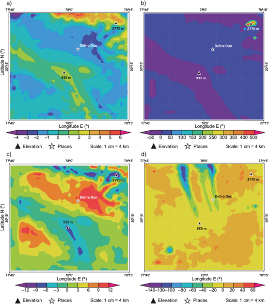
Fig. 7 Mean bias images showing the difference between modified and control run simulations. (a) Temperature bias image (in ºC) at 2 m. (b) Solar radiation bias image (in W m-2). (c) RH bias image (%). (d) Rainfall bias image (mm day^-1). 

The mean bias image (i.e., modified minus control) for temperature, ranged from -4 to 6 ºC with major values ranging from -2 to +1 ºC. The spatial temperature variation is a direct function of elevation and vegetation. The updated DEM and land boundary conditions adequately captured the process of differential heating over the surface and led to the alteration of energy fluxes contributing to the positive and negative bias in hilly regions and plains, respectively. On a spatial scale, the negative bias is predominant in the study domain, which shows that the modified run generated lesser night-time temperatures compared to the control run, reducing the well-known overestimation (night-time temperatures) issues in WRF (^{Zhang et al., 2013}). For example, the plains of Haryana, where 25% of the land cover changed to irrigated cropland in the updated land cover dataset, a temperature bias of about -2 ºC for the late evening hours and +1 ºC for early morning hours is recorded. The observed bias in temperature is attributed to changes in the thermal inertia, surface roughness, albedo and stomatal resistance associated with irrigated cropland (^{Pienda et al., 2004}). The major contributor is the low thermal inertia of irrigated cropland, since it could simulate a cooler layer in the evening and a warmer layer during the early morning. Figure 7a shows another instance where the temperature bias is very high in Shivalik hills and adjacent areas (Dehradun). The negative bias (about -3 ºC) is observed in valleys, where croplands are the predominant vegetation, and the positive bias (as high as 4 ºC) is noticed in the hilly terrain with forest cover. Forests serve as a heat-trap due to higher surface roughness and canopy cover, thus having higher nighttime temperatures than croplands (^{Lee et al., 2011}). This phenomenon is captured well by the modified run, where simulated temperatures are high (low) in forest (croplands) regions.

The difference of relative humidity (RH) at the 2-m level exhibited almost a similar pattern of spatial variation as temperature but an opposite behavior due to the inverse relationship between temperature and RH. The updated land surface boundary with distinct land cover changes in the valley and hilly areas of Uttarakhand (Fig. 7c) showed a significant difference in RH between the modified and control runs ranging from -12 to 12%, with most values falling within -6 to 9%. Earlier studies have reported underestimation (overestimation) of nighttime RH for croplands (forests). In agreement with the previous results, the negative bias is seen in the hilly forest regions and a positive bias is observed in the plains and valley areas with croplands, elucidating the improvement offered by the modified run.

The difference in solar radiation values ranged from -50 to 200 Wm^-2. Since during nighttime incoming solar radiation is not present, values are more representative of the emittance (long-wave radiation). The modified run gave slightly higher values (positive bias) in the plains and valleys, where the modified datasets improved the representation of emissivity.

Case 2 was used for evaluation of rainfall simulations. The bias in rainfall lies between -140 to 20 mm day^-1 for modified and control runs on a rainy day (from local disturbances). A positive bias of 2 to 5 mm day^-1 in rain precipitation was found across the plains, particularly in areas where agricultural land use has shifted from dry land to irrigated crop/pasture. The substantial negative bias in some regions showed that the modified run reduced the false alarm simulated by the control run. A value of 140 mm day^-1 as forecasted by the control run is very unrealistic for October in the study domain and the modified run eliminated this error. The improved roughness and moisture flux simulations in the lower boundary layer helped to reduce the unrealistic rainfall alarm in the valley (Fig. 7d). The hilly areas covered with evergreen forests showed a realistic rainfall pattern in the modified run with an increased rainfall amount due to the improved representation of orography and LAI. The increased moisture availability at lower levels would have given the potential for convergence. Although the rainfall simulation from modified runs followed a similar pattern as that of observed values by reducing false alarms, the rainfall amount is largely overpredicted for this event. Rainfall is a result of combined processes of physics and dynamics at a certain location, and land surface changes alone are insufficient to capture the entire variability (^{He et al., 2017}).

3.2 Impact of land state changes on weather forecast over selected stations

In order to evaluate the performance of the WRF model in a detailed manner, AWS at Roopanagar, Patiala and Bhatinda were considered (Fig. 6b). The selected stations represent the variability in topography and land-use of the study region. Roopnagar station exemplifies the hilly region and partly has forest cover; Patiala station is located in the transition region from the plains to the hilly zone, being mostly an agricultural area, and Bhatinda station is located entirely in the plains, belonging principally to the urban category. A grid of 10 × 10 km assessed the percentage changes of land cover in the selected stations (Table II). The influence of the land state change is evaluated based on the degree of positive/negative mean bias and associated RMSE for the forecasted weather variables from the two experiments against the actual station data at these three locations (Fig. 8). It is evident that land surface changes have a more clear and profound effect on 2-m height air temperature simulations. For Patiala station, the land use in the model’s default dataset is irrigated cropland (80%) and urban (13%), while AWiFS based land use consists of 68% irrigated cropland and 26% urban. Since there is not a profound change, temperature curves for the control and modified runs are relatively close (Fig. 8a). The relatively cooler simulated temperature during night hours in the modified run is possibly due to increased thermal inertia associated with the reduced irrigated crop areas and urban expansion. The model reproduced temperature reasonably well at the Patiala station but with a cold bias of 1.30 ºC in the modified run. A slightly high RMSE (1.32 ºC) with new land surface boundary reveals that no improvements have occurred in the temperature simulation at Patiala station for the simulated time period. At Roopanagar, deciduous forest (40%), which is the dominant land cover category, was misclassified as mixed dry/irrigated cropland (54%) in the default dataset. Thus, as a reflection, the model-simulated temperature remains high for the modified run when compared to the control run (Fig. 8b). As discussed in the previous section, the forest acts as a trap of energy and is comparatively warmer during nighttime, which is well captured in the modified run. The higher values of thermal inertia and less moisture availability due to reduced LAI, associated with the deciduous forest have led to reduced evaporative cooling and hence simulation of higher temperatures.

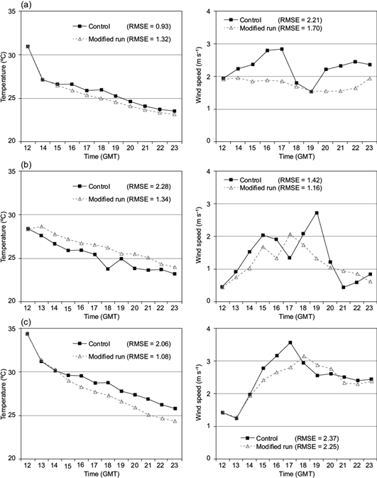
Fig. 8 Simulation of 2-m temperature and wind speed for 12-h forecast period over the three stations: (a) Patiala, (b) Ropnagar, and (c) Bhatinda. 

Table II Land cover proportion and mean bias associated with the WRF simulation for control and modified runs. 

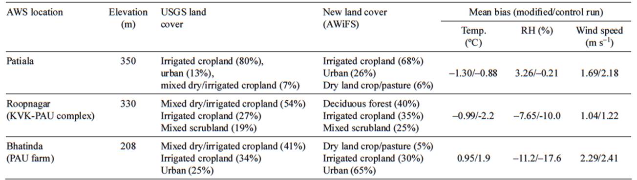
The modified run thus attempted to minimize the cold bias, and the new land boundary led to a reduction in RMSE from 2.28 ºC in the control run to 1.34 ºC at this station. Our results are in line with those reported in previous studies (^{Pienda et al., 2004}; ^{He et al., 2017}). Significant changes in land cover are observed at Bhatinda due to urbanization. Mixed dry and irrigated cropland categories in the default dataset have changed to urban land use in approximately 41%. The model predicted cooler temperatures than the control run nearly for all forecast hours (Fig. 8c), which is attributed to the lowering of nocturnal warm bias. Cooler near-surface air temperature is simulated with the new land cover because of the modulation of the surface energy fluxes through changes in the parameters (albedo, surface resistance, roughness factor, and thermal inertia). Conversion of agricultural to urban land caused an increase in surface roughness length and thermal inertia, which in turn partitioned more energy to sensible and latent heat fluxes, which subsequently cooling down the layer near the surface (^{Nicholas and Lewis, 1980}). Thus, the positive (warm) bias of temperature reduced from 1.9 to 0.9 ºC at Bhatinda by modifying the land boundary (Table II). The modified run has also decreased RMSE (1.08 ºC) compared to the control run at this site.

The modification of land boundary conditions did not show much difference in the simulated RH at Patiala, which is identical with temperature simulations. The model predicted RH agreed with observation in the control run (bias = -0.21 ºC), but a positive bias (3.26 ºC) is noticed in the modified run at Patiala (Table II). For the other two stations, the model mostly underestimated RH in both experiments, with a reduced magnitude of underestimation in the modified run. The updated model improves the prediction of RH at both stations, which is evident from the reduction in mean bias from -10 to -7.65% at Roopanagar and -17.6 to -11.2% at Bhatinda. ^{Flaounas et al. (2010)} reported similar results for RH simulations. The relatively higher humidity simulated with the new land cover could be attributed to the higher magnitude of fluxes, and more partitioning of energy to latent heat flux and sensible heat flux due to the conversion of irrigated cropland to deciduous forest or urban land cover.

Both control and modified runs produced a strong positive bias in wind speed during all the forecast hours (Table II). The simulated wind speed for both runs followed the observed wind speed patterns but largely over predicted the values (Fig. 8). ^{Zhang et al. (2013)} also observed the nighttime overestimation of wind values. We also noticed the overprediction of surface wind speed over plains and valley areas in the southwest of the study area and the underprediction over hilly regions in its northeast portion. Previous studies (^{Beljaars et al., 2004}; ^{Case et al., 2008}; ^{Jiménez and Dudhia, 2012}) have reported similar results demonstrating the tendency of the WRF model to overestimate surface winds in the plains and underestimate its values over hilly terrain. A positive bias ranging from 1.04 to 2.41 m s^-1 is noticed for all the three stations. The drag resulting from unresolved orography due to the lack of parameterization of fine roughness elements within the model is one of the primary reasons for the systematic positive bias in the model simulated wind speed (^{Jiménez and Dudhia, 2012}). Also, the improper representation of the decoupling between near-surface and above-layer air by the model leads to the over-prediction of wind speed values, especially during the nighttime (Zhang et al., 2013). The wind simulation agrees with the reports in peninsular India using the MM5 model (^{Srinivas et al., 2011}). Marginal improvement in the simulated wind speed is noticed in the modified run. The updated land state parameters have led to predictable atmospheric circulation associated with realistic heating/cooling processes over these regions.

3.3 Statistical analysis across available stations

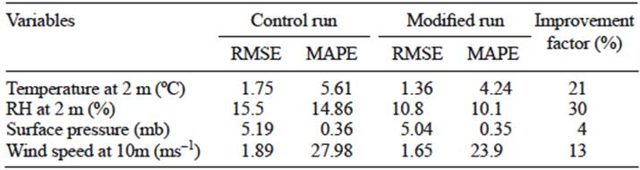
The temporal evolution of model-simulated mean weather parameters during forecast hours (beginning at 12:00 GMT) is compared to the corresponding temporal pattern of observations from a network of ISRO-AWS stations (Fig. 9). The correspondence and accuracy of the model simulations are evaluated with RMSE, MAPE and the improvement factor (Table III). The model has simulated cooler temperatures until midnight (i.e., 20:00 GMT) after which the values exceeded the observed values. The improvement factor of the modified run over the control run for surface temperature is 21% with a mean RMSE and MAPE of 1.36 and 4.24 ºC, respectively. Results are in agreement with a similar study conducted in the Indian region by ^{Srinivas et al. (2011)}. Among all variables under evaluation, RH showed the highest level of improvement during 12-h forecasts. The hourly pattern of simulated RH from the modified case closely followed the pattern of actual values. The improvement factor in RH with the altered land boundary conditions is 30%. The modified run yielded a comparatively lower RMSE (10.8%) and MAPE (10.1%) than the control run. The model underpredicted the surface pressure, but it captured the hourly trend of observed surface pressure. The values of RMSE and MAPE for surface pressure did not show much difference between the control and modified experiments. The surface winds from the model are overestimated in both simulations. The RMSE and MAPE associated to the modified run are 1.65 m s^-1 and 23.9%, respectively. An improvement factor of 13% is noticed over the control run. The results confirm that there is a specific impact on temperature and RH simulations. The feedback mechanisms are captured accurately with the near-to-real representation of the land state parameters, which has led to the increase in the quality of forecasts made by the modified run (^{Tian et al., 2004}).

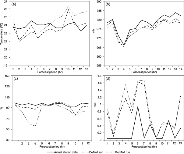
Fig. 9 Comparison between simulations and actual station data across stations for a 12-h simulation, from 12:00 to 23:00 GMT on October 1, 2008. (a) Mean temperature. (b) Pressure. (c) RH. (d) Wind speed. 

Table III Evaluation of WRF forecasts against ISRO-AWS station data. 

3.4. Evaluation of the temporal variability of near-surface variables

The updated datasets are used in the WRF model to simulate micrometeorological weather for a longer time-period of seven days (with one-day spin-up time) (case 3). The results are tabulated in Table IV, which explains the temporal evolution of RMSE for various near-surface weather variables. Appreciable results are obtained for temperature simulations especially for maximum temperatures, which are simulated close to observations (Fig. 10a). A comparatively significant error in the simulated minimum temperature shows that the model has issues in reproducing nighttime temperatures as observed in section 3.1. Minimum temperatures for starting days (March 25-27, 2009) are underpredicted, while the remaining days are overpredicted due to the dropping actual minimum temperatures after March 27, 2009. The model’s systematic bias to underestimate high temperatures and to overestimate low temperatures is very evident in this case. The RH plot (Fig. 10b) shows that the simulated values closely follow the pattern of observed values. However, the model mostly underpredicted RH. Wind speed, in general, is overestimated by the modified run (Fig. 10b) due to the unresolved decoupling between different layers of the model and radiative cooling. The modified run followed the observed rainfall patterns but underpredicted the amount of rainfall (Fig. 10c) for the simulation period. The forecast performed consistently across the lead times with an average RMSE of 2.5 ºC for maximum temperatures, 3 ºC for minimum temperatures, 2 m s^-1 for wind speed, 18% for RH and 3.5 mm for rainfall. The results are in accord with results obtained from earlier studies (Case et al., 2008; ^{Liu et al., 2008}; ^{Zhang et al., 2013}).

Table IV Day-wise RMSE values for a seven-day forecast across stations. 

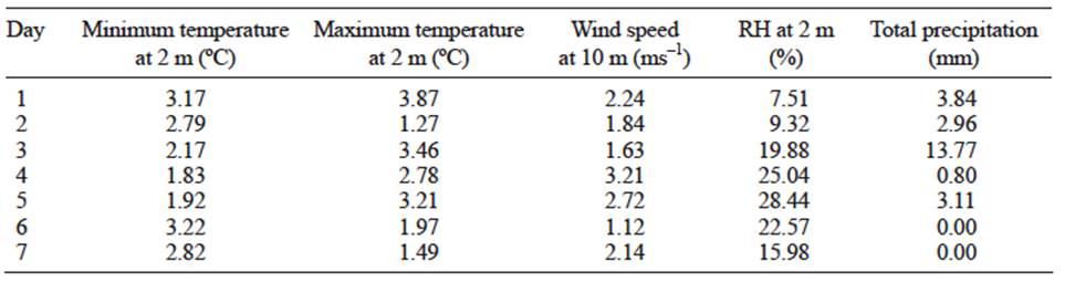
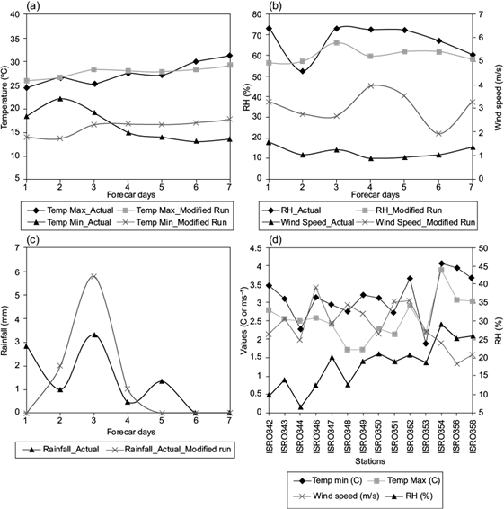
Fig. 10 Evaluation results of seven-day forecasts from March 25, 2009 to March 31, 2009. (a), (b) and (c) Variation of simulated variables (maximum and minimum temperature, RH, wind speed and precipitation with actual data). (d) RMSE variations between stations. 

Across stations, ISRO 346, ISRO 352 and ISRO 354 have large errors while ISRO 344 and ISRO 348 have fewer errors for all the simulated weather variables (Fig. 10d). Interestingly, the stations that had large errors are located in low-lying areas and predominantly have urban and fallow land-uses, while the stations with fewer errors belong to upland agricultural zones. This behavior reveals that modified datasets are useful for realistic micrometeorological weather simulations for extended time periods in vegetated areas. The significant errors in urban and fallow land uses proved that the adjusted datasets (LULC, LAI and DEM) alone are insufficient to capture the entire weather variability in those regions.