1. Introduction

Improving air quality in many large cities requires a better understanding of the sources and transformation of pollutants in the atmosphere. The air quality models constitute a major tool to carry out this task. However, the process of verifying the model results can be even more important.

The Weather Research Forecast (WRF) model was developed at the National Center for Atmospheric Research (NCAR). ^{Grell et al. (2005}) and ^{Fast et al. (2006}) updates incorporated into the WRF the chemical transformations, complex gas-phase chemistry, photolysis, and aerosols, creating in this way the WRF-chem model. In order to work with the WRF-chem model outputs, there are several computing packages: NCL (^{NCAR, 2015}); GrADS (^{COLA, 2015}); NetCDF (^{UNIDATA, 2015}); and the Unified Post-Processor (UPP), developed at NOAA (^{DTC, 2015}). All of them are very useful to visualize and extract information. Also, there are statistical tools that serve to evaluate the performance of model simulations, in some cases comparing the simulation results against observations.

Recently, the Model Evaluation Tools (MET) (^{Gotway et al., 2014}), a state-of-the-art suite of verification tools, was released by the Developmental Testbed Center (DTC) (http://www.dtcenter.org/met/users/index.php). It can perform a set of standard verification scores by comparing gridded model data with point-base observations and with gridded observations, among others. This kind of software provides useful information to the model users in order to improve the model performance by testing different model configuration setups, to improve the forecast and the decision making, and to identify forecast weakness and strengths. MET reads the output from UPP. In turn, the UPP code take in WRF output files (wrfout*) in NetCDF format. The original configuration of UPP can read several fields (eg, U, V, T, albedo) (see ^{Baldwin et al., 2012}, chapter 7, table 2). However, as far as we have seen, the chemical species oriented to the study of air quality are not included in these fields. Therefore, changes were made in the UPP source code and the MET configuration file to add new fields for air quality modeling evaluation.

In this document, a detailed description of modifications made in both UPP and MET is provided. These changes must be included to incorporate relevant chemical species (NO, NO₂, SO₂, CO, particulate matter, O₃) and meteorological parameters into the verification process. These modifications have been tested in the UPPV3.1 (http://www.dtcenter.org/upp/users/) and METv5.2 releases, under a Linux 86-64 cluster with the corresponding Fortran, C and C++ Intel compilers. A script is given in Appendix B that allows controlling the desired flow through MET. However, the process to perform the evaluation is similar to the procedure described in the WRF-NMM users page for UPP and MET.

A specific episode of high weekend ozone concentration to illustrate the verification process is considered, where MET is used to verify agreement between simulated species concentrations and data form the Red Automática de Monitoreo Atmosférico (Automatic Atmospheric Monitoring Network, RAMA) in Mexico City. The episode corresponds to the “ozone weekend effect” reported in ^{Stephens et al. (2008}), which occurs when vehicular traffic emissions decrease during the weekend; the amount of ozone measured in the monitoring stations remains approximately the same or higher that during the weekdays.

2. UPP modifications

Modifications are needed in order to incorporate new chemical species in the post-processing data from the WRF-chem model. It is essential to modify the following files:

DEALLOCATE.f, INITPOST.F , MDLFLD.f, ALLOCATE_ALL.f, RQSTLD.f , VRBLS3D_mod.f and wrf cntrl.parm. Specific line codes for each file are presented in Appendix A.

To place data in a standard grib format, run the UPP tool unipost.exe provided script in UPP (run_unipost). The WRF-Chem considers the ARW core therefore the utility copygb was not used.

3. MET modifications

MET reads gridded forecast data for both gridded and point observations. The tools interpolate gridded fields to a point observation using user specified options. Point observations may be supplied in PREPBUFR or ASCII format. In our case the ASCII observation files are re-formatted by the ascii2nc tool to create an intermediate NetCDF file for point statistics evaluation by using the Point-Stat tool. The output NetCDF file can contain meteorological and chemical variables.

Example of variables that can be incorporated in the input file for ascii2nc:

ADPSFC 76201 20130101_000000 19.635 -98.912 2240. 11 776. -9999. 1 284.150

ADPSFC 76201 20130101_000000 19.635 -98.912 2240. 33 776. -9999. 1 -0.618

ADPSFC 76201 20130101_000000 19.635 -98.912 2240. 34 776. -9999. 1 0.329

ADPSFC 76201 20130101_000000 19.635 -98.912 2240. 52 776. -9999. 1 58.000

ADPSFC 76201 20130101_000000 19.635 -98.912 2240. 180 776. -9999. 1 2000.000

ADPSFC 76201 20130101_000000 19.635 -98.912 2240. 148 776. -9999. 1 1500.000

ADPSFC 76201 20130101_000000 19.635 -98.912 2240. 232 776. -9999. 1 6000.000

ADPSFC 76201 20130101_000000 19.635 -98.912 2240. 141 776. -9999. 1 23000.000

ADPSFC 76201 20130101_000000 19.635 -98.912 2240. 142 776. -9999. 1 30000.000

ADPSFC 76201 20130101_000000 19.635 -98.912 2240. 156 776. -9999. 1 127.000

ADPSFC 76201 20130101_000000 19.635 -98.912 2240. 157 776. -9999. 1 -9999.000

The names particle matter (coarse) and particle matter (fine) are used for PM₁₀ and PM_2.5, respectively. The chemical variables are set up in different parameter table versions (^{ON388, 2013}) as shown in Table I. For the chemical variables CO, NO₂, NO and SO₂ the table version 141 has to be explicit. In order to do the comparison between model and observations in the configuration file (PointStatConfig) the following lines has to be modified. For meteorological variables temperature, u wind, v wind and relative humidity there is no need to set the grib table:

Table I Chemical species description and grib table version and code 

Note: μl m^-3 = ppb.

field = [

{

name = “TMP”;

level = [ “L1” ];

cat_thresh = [ >273, >288, >293 ];

},

{

name = “UGRD”;

level = [ “L1” ];

cat_thresh = [ >=2 ];

},

{

name = “VGRD”;

level = [ “L1” ];

cat_thresh = [ >=2 ];

},

{

name = “RH”;

level = [ “L1” ];

cat_thresh = [ >=30 ];

},

for chemical compounds and particles, O₃, NO, NO₂, CO, SO₂, PMTC and PMTF :

{

name = “OZCON”;

level = [ “L1” ];

cat_thresh = [ >=50, >=110 ];

GRIB1_ptv = 129;

},

{

name = “NO”;

level = [ “L1” ];

cat_thresh = [ >=105, >=210 ];

GRIB1_ptv = 141;

},

{

name = “NO2”;

level = [ “L1” ];

cat_thresh = [ >=105, >=210 ];

GRIB1_ptv = 141;

},

{

name = “CO”;

level = [ “L1” ];

cat_thresh = [ >=5500, >=11000 ];

GRIB1_ptv = 141;

},

{

name = “SO2”;

level = [ “L1” ];

cat_thresh = [ >=65, >=130 ];

GRIB1_ptv = 141;

},

{

name =”PMTF”;

level = [ “L1” ];

cat_thresh = [ >=65, >=130 ];

GRIB1_ptv = 129;

},

{

name =”PMTC”;

level = [ “L1” ];

cat_thresh = [ >=65, >=130 ];

GRIB1_ptv = 129;

{

];

For a demonstrative purpose, gas pollutants categorical threshold values were set on the 1-h average air quality standard (upper value) and half of the standard (lower value).

4. Results

A high weekend ozone episode was considered to show a comparison between model and observed data by using MET and UPP modified codes. The episode took place in Mexico City from 06:00 LT on April 13, 2007 through 03:00 LT on Apr 15, 2007. During that period, measurements of criteria pollutants were made by RAMA. Although it is possible to extract the model formaldehyde concentrations during this episode, this compound was not measured.

WRF-chem was configured to use the chemical mechanism RADM2 as the chemical module (^{Stockwell et al., 1990}). The emissions inventory was gridded based on the National Emission Inventory for the Mexico City Metropolitan Area (MCMA) for the year 2006 (^{SMA, 2015}). These emissions were updated to fill in a 3-km spatial resolution and simulations were carried out for a 40-h time period. Finally, the observational data, required by MET, is provided by the MCMA monitoring stations (RAMA). Figures 1 and 2 show examples where simulations are compared against monitoring stations data.

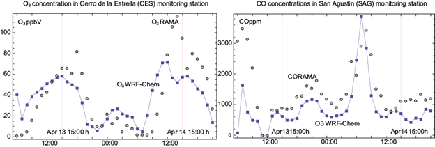
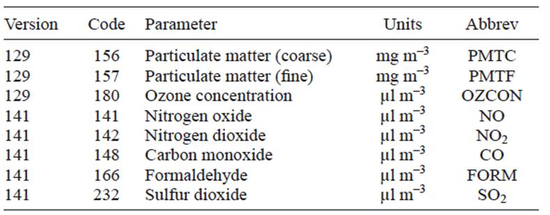
Fig. 1 Simulated and observed fields in ground based stations in Mexico City, from April 13, 2007 at 6:00 LT to April 14 at 03:00 LT. Filled circles correspond to measurements from the ground-based Air Quality Monitoring Network (RAMA) in the MCMA and lines (filled squares) are the simulations made with WRF-chem model 

Fig. 2 Simulated and observed averaged fields, from April 13, 2007 at 6:00 LT to April 14 at 03:00 LT, in Mexico City. Continuous line represents the average field calculated with the WRF-chem model, and filled circles represent the average measured field from RAMA in the MCMA. 

The Point-Stat tool computes several statistics to evaluate the forecast performance in monitoring stations. Figure 1 shows the simulated and observed concentrations of O₃ and CO in ground-base stations. To the left, the ozone concentration in the Cerro de la Estrella (CES) monitoring station is shown. The simulations (continuous line with fill squares) fit well with the observation data (filled circles) in most of the time domains, except for the high ozone concentration time interval, where the simulations underestimate the ozone peak (Apr 14, 15:00 LT). Conversely, illustrated on the right side of Figure 1, the simulated CO concentrations at San Agustín (SAG) monitoring station are well fitted in the high measured ozone concentrations. The CO simulated concentrations systematically underestimate the measurements, but almost follow the same observed data pattern, which could indicate that the emission inventory should be modified in that case. Also it is possible that MET computes the grid average of fields; the Stat-Analysis tool provides verification statistics for a matched forecast and observation grid.

Figure 2 shows the point averages of the observations and simulations, the simulated variables (continuous line with fill squares) are compared against the average of all RAMA stations (filled circle). On the left in figure 2, the average ozone concentration against RAMA data is shown. The maximum ozone concentration occurred at 15:00h Apr 14 (Saturday) and is pretty close to 140 μL m^-3 (ppbv), this value is bigger than the previous day maximum Apr 13 (Ozone weekend effect). The ozone numerical simulation concentrations underestimate the second ozone peak; the model concentration value is approximately 42% of the measured value. This pattern is presented in other monitoring stations indicating that the model underestimates the ozone concentration. In figure 2 (right panel) the average SO₂ concentration for model and observations is shown. This chemical species is well reproduced by the model especially in the first hours of the high concentration episode.

Ambient concentrations depend on the emissions and weather conditions. In the studied episode, primary pollutants (CO and SO₂) concentrations have a better agreement with the measurements than secondary pollutants (O₃). The O₃ concentration depends on primary pollutants like NO₂ and Volatile Organic Compounds (VOC), and the highest ambient concentration is reached downwind from its precursor emissions. Because CO and SO₂ concentrations from the model are in agreement with measurements, and they are primary pollutants that depend on local emissions, the high O₃ concentrations on April 14 suggest that this pollutant was transported from elsewhere.

Additionally, Table II shows examples of several verification measurements for SO₂, including the normal and bootstrap lower and upper confidence limits (NCL, BCL, NCU and BCU). In this case the threshold concentration were 130 ppb in order to compute the categorical statistics. The first parameter shown on this table correspond to the accuracy (ACC) contingency parameter. In our simulation ACC = 0.883, meaning the fraction of forecast that was correct, ACC ranges from 0 to 1, perfect forecast has an ACC value of 1.

Table II Statistical analysis results for SO₂ evaluation. Accuracy (ACC), Hansen-Kuipers Discriminant (HK) and Heidke Skill Score (HSS) for 662 total observations. 

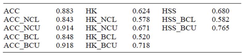
The two other parameters are the Hanssen-Kuipers Discriminant (HK) and the Heidke Skill. Its values range from -1 to 1. A perfect forecast has HK = 1, and a value of 0 indicates no skill. HSS is a skill score based on accuracy with values ranging from −∞ to 1. A perfect forecast will have an HSS = 1. For a more comprehensive description of these and other verification measurements, see Appendix C, Verification measures on the MET Users Guide v5.2.

5. Conclusions

The modifications made in the UPP code can provide files that include pollutant concentration variables (i.e., O₃, CO, SO₂, PM₁₀ and PM_2.5, among others); these files can be used by MET in order to evaluate objectively the model performance with a set of statistical parameters. A demonstration of the functionality of the code modifications was presented through its application in the case study, which showed that CO and SO₂ model concentrations have a better agreement than O₃ when compared to measured values. In the case of O₃, the first day presents a good agreement, but for the second day its concentrations could indicate that it comes from elsewhere.

These code additions can reduce the time for data analysis and standardize the evaluation procedure for chemical and meteorological variables by using a state-of-the-art suite of verification tools.