1. Introduction

Flood frequency analysis (FFA) is the basis for planning and designing bridges, culverts and flood control structures (Chow et al., 1998). The maximum capacity of these structures is defined by the design flow, which is the annual peak flow (APF) with a certain probability of being exceeded at least once during operation. This probability is known as risk and is usually expressed as a return period. Furthermore, this probability is selected by considering the economic, social and environmental effects that would be produced by the failure of the structure. Therefore, precise design flow estimates are important when evaluating the feasibility of a structure. However, due to stream flow variability, the precision of the estimates is drastically reduced when small samples are used in a conventional FFA.

Conventional estimates of the design flow are achieved via a frequency analysis of the APFs measured over a long period at a single gauging station. Assuming that the APFs are independent and identically distributed (IID), a relation between their magnitudes and non-exceedance probabilities can be achieved by fitting a cumulative probability function (CPF).

A regional flood frequency analysis (RFFA) is a well-known option for reducing the uncertainty in quantile estimates when sufficient and homogeneous data are available. A RFFA requires all available information from neighboring sites to obtain at-site estimates for a specific return period. Several previous papers have described the advantages of RFFA methods. ^{Darlymple (1960)} first introduced the index flood method. ^{Chander et al. (1978)} suggested a regional box-cox transformation. ^{Wallis (1980)} proposed the use of regional probability weighted moments. ^{Boes et al. (1989)} considered the Weibull distribution as a regional distribution. Moreover, ^{Hosking and Wallis (1993)} introduced select discordancy, heterogeneity and fitting measures. ^{Cunnane (1998)} suggested using the station-year method, whereas ^{Sveinsson et al. (2001)} proposed the population index flood method. The method introduced by ^{Hosking and Wallis (1993)} appears to display more acceptability in RFFA; its application can be found in ^{Lim (2007)}, ^{Saf (2009)}, ^{Notto and Loggia (2009)}, ^{Hussain (2011)}, and ^{Rostami (2013)}.

Other options to reduce the uncertainty in estimating quantiles are "transfer methods". ^{Zaidman et al. (2003)} suggested two methods to transfer information from a donor basin to an object basin. In the first method, the standardized shape of the donor CPF is transferred. In the second method, the plotting positions of the events, occurring over the same period of time (year), are transferred. ^{Dong et al. (2013)} introduced a non-parametrical transfer method that uses an iterative procedure to gradually approximate the optimal CPF.

This paper proposes a new approach to reduce the uncertainty in the estimation of APF quantiles resulting from small sample sizes, and to dispense with neighboring information. This approach consists of simulating multiple APF samples to achieve a more accurate frequency distribution. To improve the accuracy, these synthetic samples must be conditionally simulated from a steadier variable. In this paper, APF samples are conditionally simulated using the annual mean flows (AMFs).

Hydrometric information from 13 gauging stations located in the Susquehanna River basin was employed in this study. APF quantiles were estimated according to the following methods: (1) a conventional FFA method, (2) a station-year method, and (3) the proposed method. The uncertainty of each method was measured by computing the coefficients of variation (CV) between the quantiles estimated from 10-, 20-, 30-, 40- and 50-year subsamples with those obtained from historical information.

2. Materials and methods

2.2 Data

The stream flow time series used in this study were obtained from the National Water Information System of the United States (^{NWIS, 2015}); 13 gauging stations in the Susquehanna River basin were selected. The locations of the study sites are shown in Figure 1.

Fig. 1 Location of the gauging stations used in this study. 

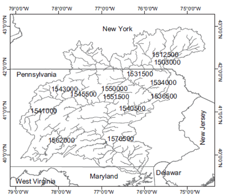
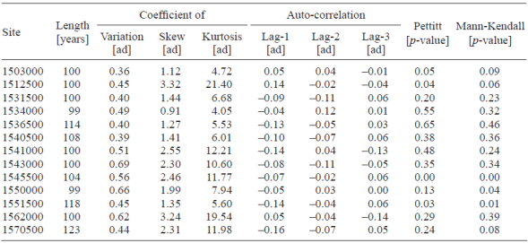
To evaluate the independence of the series, the autocorrelation functions (ACFs) were contrasted with the limits proposed by ^{Anderson (1942)}. To identify possible non- homogeneities, such as change points or trends in the time series, the ^{Pettitt (1979)} and Mann-Kendall tests (^{Kendall, 1938}; ^{Mann, 1945}) were performed. A brief description of the series and the results are summarized in Table I.

Table I Selected characteristics of the annual peak flow series. 

2.3 Conventional FFA method

Let X represent the APFs and X = {x₁,...,x_n} be a sample of X at any site in the study region. Then, a conventional FFA method for APF quantile estimation can be defined as follows:

Step 1: Sort in ascending order X,i.e.,X=x1≤⋯≤xn.

Step 2: Obtain the empirical non-exceedance probability of each x ₍₁₎ in X, i.e., Pr[X≤ x _(n)], using the Weibull's plotting position formula:

p(i)=in+1 (1)

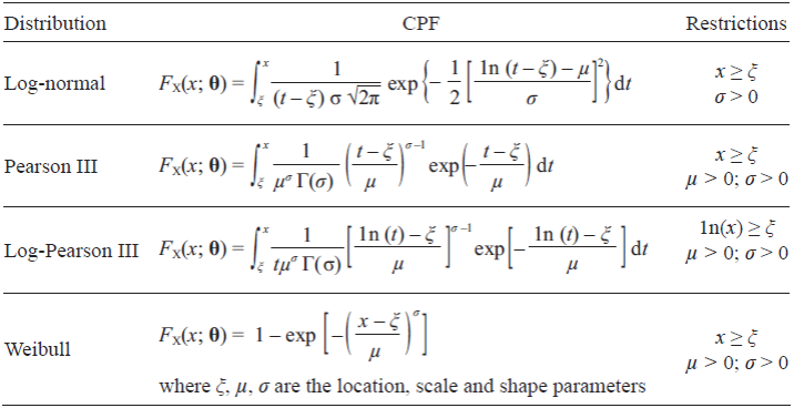
Step 3: Estimate a theoretical CPF of X, i.e., Pr[X ≤ x] (from Table II), by minimizing the sum square error (SSE) of the sample quantiles:

SSE=∑i=1nxi-xpi2 (2)

Table II CPFs applied in the conventional FFA for this study. 

where xpi=infx∈R:pi≤Fx;θ.

Step 4: Select (as the best CPF of X) the CPF with the smallest standard error of fit (SEF) (^{Kite, 1988}) using the following relationship:

SEF=SSE/k-1 (3)

where k is the number of distribution parameters.

Step 5: Estimate the quantiles of X as xq=infx∈R:q≤Fx;θ[/p]

2.5. Proposed method

Let Y represent the AMFs, Y = {y₁,..., y_n} be a sample of Y at any site in the study region, X represent the APFs and X = {x ₁,..., x _n} be a sample of X at the same site over a consistent recording period. The proposed method for APF quantile estimation utilizes the following steps:

Step 1: Sort Y in ascending order, i.e., Y=y1≤⋯≤yn maintaining each x _t occurring at the same time t as y _(t). Thus, an empirical relation y1,xt1,...,yn,xtn can be defined.

Step 2: Obtain the APF ratios Θ {θ ₁,..., θ _n} by dividing each x _t by its corresponding y _(i), i.e. θi=xti/yi. Thus, an empirical relation y1,θ1,...,yn,θn can also be defined.

Step 3: Apply the conventional FFA to Y to determine the best CPF of Y, i.e., F(y; θ).

Step 4: Generate 100 000 random synthetic AMF defined as yu=infy∈R:u≤Fy;θ by sampling u from a continuous uniform distribution, i.e. u~U[0,1].

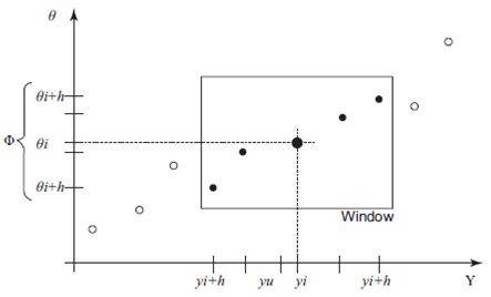
Step 5: For each generated y(u), find its closest y _(i) in Y and its corresponding θ _i in Θ. Then using a window of size h = [n ^2/3] centered on y _(i), define Φ={ϕ ₁ ,... ϕ _m} as a subsample of Θ , where ϕ ₁= θ _max(1,i+h) and ϕ _m= θ _max(n,i+h) (Fig. 2). The specific window size was obtained after a trial and error process. It was observed that a window of this width provides a reasonable balance between flexibility and precision of the results.

Fig. 2 Window centered on the closest generated AMF. 

Step 6: Assume that every ϕ _j in Φ are equally likely to occur, i.e., Pr[ϕ = ϕ _j]=1/m, and extract (from each Φ) a ϕ value, such that ϕ(ʋ)=sup{ϕ _j ∈ Φ; ʋ ≤ j/m) by sampling v from a continuous uniform distribution, i.e., ʋ~U[0,1].

Step 7: Multiply each generated y(u) by the extracted ϕ(ʋ), i.e., x(y) = x(u) ∙ ϕ(ʋ).

Step 8: Estimate the quantiles of X as the q-th percentiles of the generated x(y).

3. Reliability of the methods

To evaluate the uncertainty in the estimated quantiles determined using the former methods, historical quantiles were first estimated from historical information. Then, different scenarios of available information were simulated by extracting 10-, 20-, 30-, 40- and 50-yr subsamples, and new quantiles were estimated. Finally, the coefficient of variation of the quantiles estimated from the 10-, 20-, 30-, 40- and 50-yr subsamples were computed using the following expression:

where x-mj (q) and Smj (q) are the mean and standard deviation of the q-th quantiles xi,mj (q) estimated from each subsample i of size m at site j, respectively, and x^j (q) are the q-th quantiles estimated from the historical information available from the same site j.

4. Results and discussion

The CV values for each subsample size (10, 20, 30, 40 and 50 years) by applying (1) the conventional FFA method, (2) the station-year method and (3) the proposed method were computed and contrasted.

Concerning all 13 study sites, approximately 200 CV values were computed for different q-th quantiles from each subsample size. Therefore, nearly 1000 CV values for each return period were computed for each method.

The variations in the set of estimated quantiles for the shortest length of records (i.e., 10 years) are shown in Figures 3-⁷. In these figures, the 50th per-centile is the median of the estimates, and the 10th and 90th percentiles are considered as lower and upper bounds, respectively. These figures show that the proposed method generates the narrowest limits compared with those obtained using the conventional FFA approach.

Fig. 3 Quantiles obtained from 10-yr subsamples at stations 1503000, 1512500 and 1531500. 

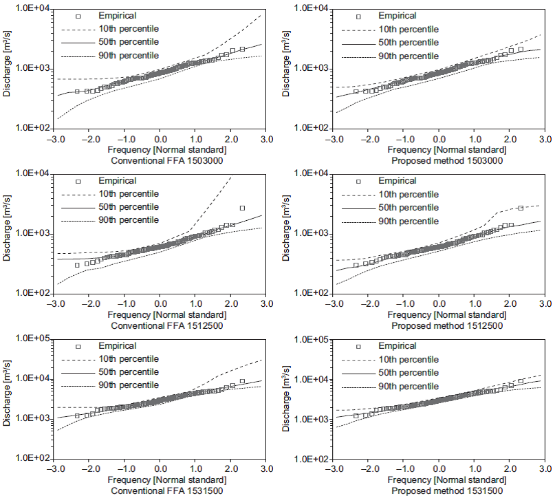
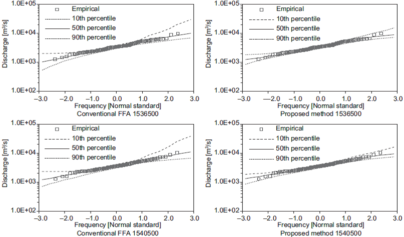
Fig. 4 (Continued) Quantiles obtained from 10-yr subsamples at stations 1503400, 1536500 and 1540500. 

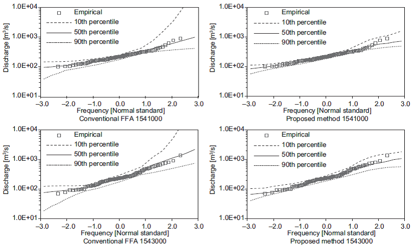
Fig. 5 Quantiles obtained from 10-yr subsamples at stations 1541000, 1543000 and 1545500. (Continue) 

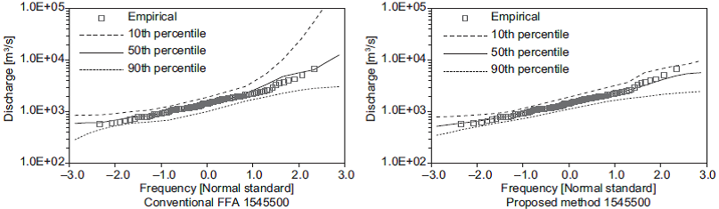
Fig. 5.(Continued) Quantiles obtained from 10-yr subsamples at stations 1541000, 1543000 and 1545500. 

Fig. 6 Quantiles obtained from 10-yr subsamples at stations 1550000, 1551500 and 1552000. 

Fig. 7 Quantiles obtained from 10-yr subsamples at stations 1541000, 1543000 and 1545500. 

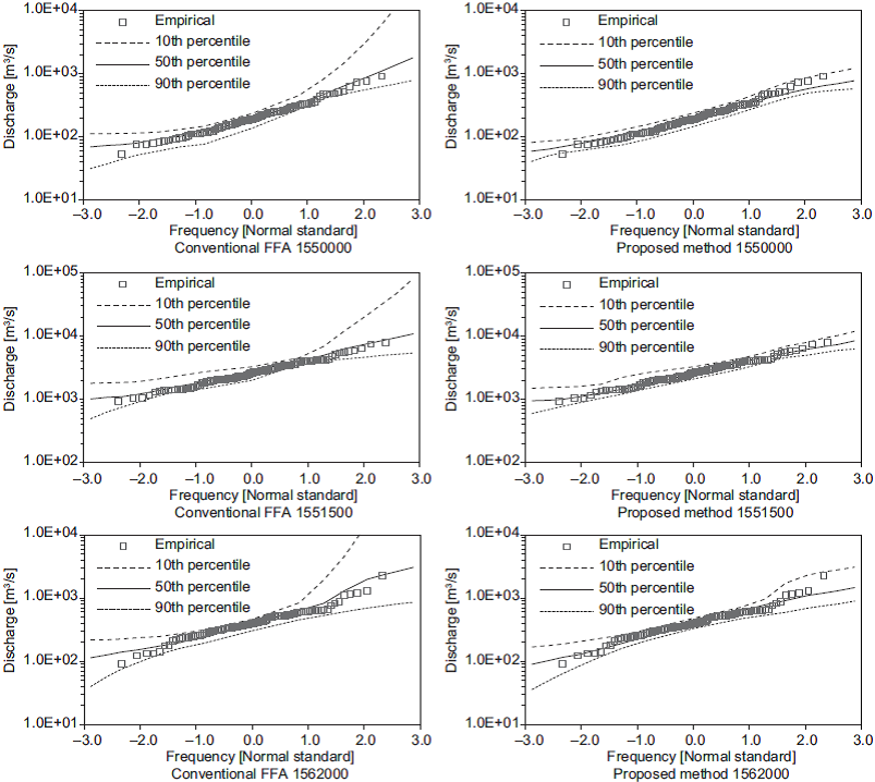
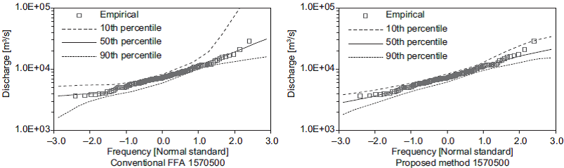
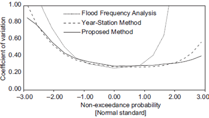
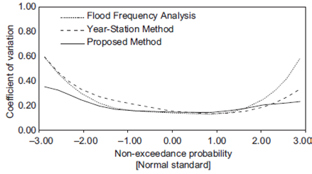
In general, lower CV values were obtained in 71% of the cases using the proposed method instead of the conventional FFA method. Lower CV values were obtained for a return of approximately two years in 33% of the cases, whereas 99% of the cases showed lower CV values for return periods exceeding 100 years.

Furthermore, in 67% of the cases, lower CV values were obtained using the proposed method instead of the station-year method. In 50% of the cases, lower CV values were obtained for a return period of approximately two years, whereas lower CV values were found for return periods exceeding 100 years in 93% of the cases.

The geometric means of all CV values for the same return period obtained from (1) the conventional FFA, (2) the station-year method and (3) the proposed method are contrasted in Figures 8-¹².

Fig. 8 CV obtained using 10-yr subsamples. 

Fig. 9 CV obtained using 20-yr subsamples. 

Fig. 10 CV obtained using 30-yr subsamples. 

Fig. 11 CV obtained using 40-year subsamples. 

Fig. 12 CV obtained using 50-yr subsamples. 

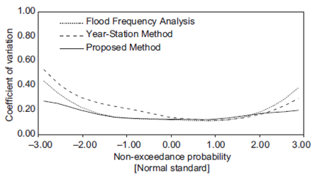
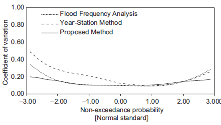
5. Conclusions

A new approach for estimating APFs for different return periods is presented in this study. This approach consists of a conditional simulation process of synthetic samples of APFs and AMFs to achieve the frequency distribution. Thirteen gauging stations located in the Susquehanna River basin, which is along the east coast of the United States, were used in this study.

To evaluate the proposed method, the uncertainties in the quantiles estimated using (1) a conventional FFA, (2) a station-year method and (3) the newly proposed method were compared by computing.

The results indicated that the quantiles estimated using the proposed method varied less than those estimated via the conventional FFA, especially when they were estimated from 10-yr subsamples and for return periods exceeding 100 years. Therefore, the proposed method can reasonably reduce the uncertainty in quantile estimation from small sample sizes.

The results also showed that the quantiles estimated using the proposed method are equal or less than those computed by the station-year method, even if only a third of the information is used.

The analysis also demonstrated that the proposed method performed adequately when quantiles were estimated from the gathered samples. Moreover, more flexible frequency distributions were simulated using the proposed method than with the conventional frequency distributions.