Assessing interannual water balance of La Plata river basin

 

C. M. KREPPER
Consejo Nacional de Investigaciones Científicas y Tecnológicas de Argentina–Facultad de Ingeniería y
Ciencias Hídricas, Universidad Nacional del Litoral, Santa Fe, Argentina

V. VENTURINI
Facultad de Ingeniería y Ciencias Hídricas, Universidad Nacional del Litoral, Santa Fe, Argentina
Corresponding author; e–mail: vventurini@fich.unl.edu.ar

 

Received May 22, 2009, accepted September 11, 2009

 

RESUMEN

El río Paraná es el más importante de la Cuenca de La Plata, sustentando economías regionales en tres países. Durante las últimas décadas, se han producido cambios significativos en la cuenca del Paraná, debido a la deforestación y sustitución de cultivos. Esto pudo haber modificado la respuesta de la cuenca en términos de caudales del río Paraná. El objetivo principal de este trabajo es analizar la estructura de la serie temporal de evapotranspiración (ET(t)) de la Cuenca Superior del Paraná. En primer lugar se estudió la relación entre las variables en la ecuación del balance hídrico y luego se aplicó un análisis de espectro singular (SSA, por sus siglas en inglés) para determinar las señales presentes en las series de ET(t). El estudio de correlación muestra que ET(t) está correlacionada con las precipitaciones en las subcuencas del norte y no está correlacionada en la más austral. Las series temporales ET(t)₁ ET(t)₃ y ET(t)₄ muestran una señal de baja frecuencia mientras que las señales dentro del rango ENSO son estadísticamente significativas en ET(t)₁, y ET(t)₄ , aunque están presentes en las otras subcuencas (ET(t)₂, y ET(t)₃)como señales débiles. En la Cuenca de La Plata ET(t) estaría afectada tanto por los cambios en las propiedades físicas de la cuenca como por la presencia de la señal en el rango ENSO de las precipitaciones.

 

ABSTRACT

The Paraná river is the most important component of the La Plata basin, sustaining regional economies in three countries. In the last decades, significant regional changes such as deforestation and crop substitution have been taken place in the Paraná basin. This fact could have modified the basin response in terms of the Paraná streamflow. The main objective of this paper is to analyze the structure of the evapotranspiration (ET(t)) time series of the upper Paraná basin. We analyzed the relationship between the variables in the water balance equation, then we applied a singular spectral analysis (SSA) to learn more about the temporal structure of the ET(t) time series. The correlation study shows that ET(t) is correlated with precipitations in the northern sub–basins but it is not correlated at all in the southern basin. The time structure of ET(t)₁ ET(t)3 and ET(t)₄ exhibit low–frequency signals while the ENSO–range signals are statistically significant in ET(t)₁ and ET(t)₄ although it also appears in ET(t)₂ and ET(t)₃ as a weak signals. Looking at the whole basin, ET(t) would be affected either by changes in the basin physical properties or by the ENSO–range signals present in precipitation.

Keywords: La Plata basin, water balance, SSA, evapotranspiration.

 

1. Introduction

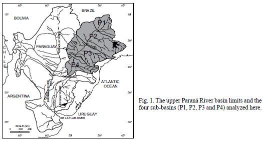
The Paraná River is the most important component of the La Plata river basin (LPB) system and, together with the Paraguay river form a combined basin that covers an area of around 2.6 x 10⁶ km². The Paraná–Paraguay basin represents around 84% of the total LPB and contributes more than 80% to the La Plata river streamflow. The Paraná river basin, upstream of the city of Posadas (Fig. 1) is known as the upper Paraná basin (Krepper et al., 2008), and covers an area of around 993,360 km², where 89.6% of the drainage area is located in Brazil and the remains in Paraguay and Argentina.

During the austral summer in South America, the South Atlantic convergence zone and a convective activity in the Amazon basin are the main components of the South American Monsoon System (SAMS) (Carvalho et al., 2004), and an important source of precipitation for southeastern South America. The northern portion of the Paraná basin has the largest precipitation contribution during austral summer with dry conditions during the cold season as a result of the predominant effects of the SAMS (Grimn et al., 1998; Berbery and Barros, 2002). Toward the south, the annual cycle changes in a transitional zone where no unique seasonal maximum is found. Large contributions in precipitation occur in the late winter and spring season. In this region, during the austral cold season, the most relevant forcing is due to frontal penetration, associated with migratory extra tropical cyclones (Vera et al., 2002). Annual mean rainfall in the LPB tends to decrease from north to south and from east to west. During the second half of the twentieth century, important positive trends in annual precipitation in almost the entire south american region, between 22° and 45° S to the east of the Andes was reported by several authors (Castañeda and Barros, 1994, 2001; Minetti and Vargas, 1997; Krepper and Sequeira, 1998; among others). On the other hand, discharges of the most important rivers in the LPB had positive trends since early 70s. García and Vargas (1998) have inferred that during the last century the Paraná River at Posadas had two very different periods: a driest period between 1931 and 1970, with a mean annual streamflow of 10,972 m³/s and a humid period after 1970 with 14,495 m³/s. Tucci and Clarke (1998) pointed out that increasing runoff after the 70s may be due to rainfall increases, agriculture practices or both. They conclude that if rainfall has been the principal cause of increased runoff, the increase may not be permanent; but if changes in the land use have contributed to increase runoff, it is possible that such effect may be more permanent. Krepper et al. (2008) investigated aspects of the temporal structure of time series of Paraná river flow upstream of Posadas. From a detailed analysis at sub–basin scale, they showed that not all the signals present in precipitation are reflected in streamflow series contributions. The sub–catchment responses to precipitation have strong sub–basin dependence. In general, changes in mean annual discharge, for the different sub–basins of the upper Paraná basin, could not be explained by increases in precipitation, especially downstream of Jupiá.

For the southeastern South America region the detected trends, in mean annual temperature have been on the order of +0.6 or +0.8 °C from 1976 to 2000 (IPCC, 2001). Marengo and Camargo (2007) have analyzed air temperature in Southern Brazil for the 1960–2002 period. They reported, at annual scale, significant trends for minimum temperature that show rates of warming ranging between +0.5 and +0.8 °C per decade, while the maximum temperature show smaller increase trends. Consequently, the diurnal temperature range exhibits negative trends in the region for 1960–2002.

Several authors have mentioned that significant regional changes in deforestation and crop substitution have taken place in the Paraná basin (Anderson et al., 1993; Tucci and Clarke, 1998; Schnepf et al, 2001). The final result is that destruction and degradation of the original Atlantic rainforest, has been severe during the last decades. Today only about 7–8% of the original forest, which formerly covered more than 1'200,000 km², remains pristine (Le Breton, 1998). According to Tucci and Clarke (1998), if changes in land use have contributed to modify the runoff probably such effect would be semipermanent, or at least a long–term effect. Other studies have focused on the water cycle simulation for different basin and vegetation scenarios (Li et al., 2007; Wang and Eltahir, 2000). This type of simulations suggests that climate change and land–use change have long–term impact on the water cycle. The balance between precipitation and evapotranspiration, as well as the stream flow, are modified by climate and vegetation long–term changes. Numerical simulation commonly needs several basin parameters to represent the water balance on the system. On the other hand, time series analysis is only based on the historical records of the studied variables without extra information about the basin itself.

The main objective of this paper is to assess the interannual river response at sub–basin scale and the time series structure of evapotranspiration, ET(t), of the upper Paraná basin. As a first approximation, an annual water balance equation was applied at the sub–basin scale (Fig. 1) to obtain the evapotranspiration time series (ET(t)) as a residual of the equation.

The paper is organized as follows. Section 2 describes the study area and data sources. Section 3 the method of analysis. The responses of the different sub–basins along the upper Paraná river are described in section 4. Section 5 presents a discussion of the results and the concluding remarks.

 

2. Study area and data

2.1 Study area

The Paraná river basin, upstream of the city of Posadas (shaded area in Fig. 1) is known as the upper Paraná basin (Krepper et al., 2008). It covers an area of around 993,360 km², where 89.6% of the drainage area is located in Brazil and the remains in Paraguay and Argentina.

The headwaters of the Paraná river are located in the Santa Marta and Das Piloes hills, where it takes the name Paranaiba river. The regional toponymy recognizes the name of the river as Paraná downstream of the confluence of the Paranaiba and Grande rivers. The main tributaries of the Paraná river come from the east of the basin, such as the Grande, Tieté, Paranápanema, Ivaí and Iguazú rivers; from the west, the basin receives contributions of many smaller rivers (García, 2000). The whole upper Paraná river basin was divided into four different drainage areas or sub–basins (Fig. 1): P1–basin (171,000 km²) upstream of Sao Simao, on Paranaiba river; P2–basin (306,885) formed by the drainage area between Ilha Solteira and Jupiá; P3–basin (352,695) between Itaipú and Jupiá and P4–basin (102,780) between Posadas and Itaipú.

2.2 Data

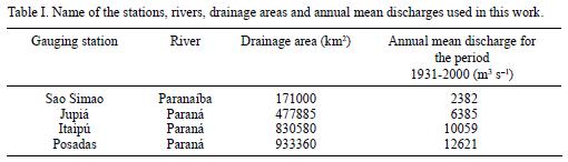
Four gauging stations (Sao Simao, Ilha Solteira, Itaipú and Posadas) on the Paraná river with 70 years of naturalized monthly discharge data (1931 –2000) were used in the present study. Brazilian monthly discharge series were obtained from the Operador Nacional do Sistema Eléctrico (ONS) do Brazil and monthly data at Posadas came from the Argentinean Subsecretaría de Recursos Hídricos (SHR). The name of the station, river as well as drainage area, the annual mean discharges and the percentage of contributions respect to Posadas mean discharge, are shown in Table I.

There are more than fifty dams along the Paraná river system, each with more than 1 km³ volume (Comisión Mixta Paraguayo–Brasileña, 1974); however, their effects on mean yearly flows are negligible (García and Vargas, 1996).

The runoff contribution of each sub–basin Q(t)j (j = 1,...,4) is determined as the difference of discharges between the corresponding gauging stations.

Precipitation data come from 0.5 x 0.5° gridded data set CRU TS 2001 available at http://www.cru.uea.ac.ik/. A significant data base, for the region, of monthly rainfall time series (more than 1100 stations) were collected, reformatted and quality–checked during the Project "Assessing the Impact of Future Climatic Change on the Water Resources and Hydrology of the Río de La Plata Basin, Argentina, 1995–1999" (Conway et al., 1999). The rainfall series were cross–checked with those in CRU global data set (Hulme, 1994) and all the new stations were added to the global data set and new time series of gridded rainfall for 1901–1995 were constructed for the region (CRU TS 1.0: New et al., 2000). The grids were subsequently updated and extended to 2000 (CRU TS 2.0: Mitchell et al., 2004), and after that to 2002 (CRU TS 2.1: Mitchell and Jones, 2005).

The data set used contains monthly precipitation records from January 1901 to December 2000 (1200 time points) for 234 grid points (upper Paraná basin). The data were summed from monthly to annual precipitation values. The precipitation grid allows us to calculate the areal average of annual precipitation rates, PR(t)_j (j = 1,... ,4), defined as the annual precipitation contribution over different sub–catchments, which we express in m³ s^–1, between 1901 and 2000.

 

3. Method of analysis

The annual rainfall is partitioned into ET and surface runoff. ET includes interception loss and the surface runoff is generated when soil water storage in the basin exceeds its capacity (Manabe, 1969; Milly, 1994; Jothiyangkoo et al., 2001). In general, volumetric water balance for a period of time shorter than a year is given by:

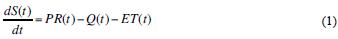
where S(t) is the volume of soil water storage, PR(t) is the precipitation rate, Q(t) is the saturation excess runoff rate and ET(t) the evapotranspiration rate.

Equation (1) is valid at different time scales, i.e. daily, monthly, seasonal, etc. The left–hand–side is significantly different from zero during short time scales. In such cases, the quantification of the water balance requires the knowledge of many parameters. On the other hand, for a long period of time, dS(t)/ dt can be considered negligible and the balance can be equated to zero (Sokolov and Chapman, 1974; Brutsaert, 2005). Thus, assuming that the annual streamflow Q(t), is assembled by the sub–surface flow, overland runoff and groundwater, and that dS(t)/ dt is negligible compared with the magnitude of the other variables over a year, the annual water balance can be written as (Brutsaert, 2005):

where PR(t) is the precipitation rate, Q(t)_j the annual runoff, ET(t) the evapotranspiration rate. The evapotranspiration rate for each sub–basin, ET(t)_j ( j = 1,...,4) , can be obtained from (2), in terms of precipitation rate for each sub–basin, PR(t)_j , in the form:

These variables were analyzed using the (SSA) method. This is a statistical method related to Principal Component Analysis (PCA), but it is applied in the time domain. The objective is to describe the variability of a discrete and finite time series in terms of its lagged autocovariance structure (Vautard and Ghil, 1989; Ghil and Vautard, 1991; Plaut and Vautard, 1994; Ghil and Yiou, 1996). For a standardized time series X(t_i), where the sample index i varies from 1 to N, and a maximum lag (or window length) is M, a Toeplitz lagged correlation matrix is formed by:

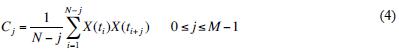
The eigenvalue decomposition of the lagged autocorrelation matrix, C_j, produces temporal–empirical orthogonal functions T–EOFs (eigenvectors), and statistically independent temporal–principal components T–PCs, with no presumption as their functional form. Each T–PCs has a variance λ₅ (eigenvalue) and represents a filtered version of the original series, which can be classified essentially into non–linear trends, deterministic quasi–oscillations and noise. A significance test for the singular values, λ₅, can be made against a red noise null–hypothesis using a Monte Carlo method, generating an ensemble of 1000 independent realizations (Allen and Smith, 1996).

 

4. The response of the upper Paraná basin

According to Conway (2001), the change in the runoff coefficient, R(t)=Q(t)/PR(t), may be a consequence of physical changes in the catchment through several mechanisms, such as changes in land–cover and land–use, in moisture availability, in evaporative demand or in rainfall characteristics. Thus, a SSA analysis on the R(t) and ET(t) series should uncover different climate and non climate effects.

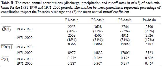
Table II shows the mean annual streamflow, contribution, , and the mean annual runoff coefficient of each sub–basin, (j =l,–––,4)forthe 1931–1970and 1971–2000 periods, according to García and Vargas (1998). We can observe from Table II an increase in and , from one period to other, especially for P3–basin, where the change in is around 71%. Nevertheless, the change in is only around 6%. At the same time remains quite constant and decreases from one period to other.

During the 1931–1970 period, the drainage area between Itaipú and Jupiá (P3 –basin) contributed with 25% of the mean discharge at Posadas station; while, after 1970 the contribution change to 34%. The change in mean annual runoff responses of P3–basin, , could not be explained by the increase in the corresponding mean annual precipitation rate, , because .

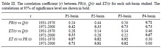
For each sub–basin, the relationship between components of Eq. 3 for the 1931–1970 and 1971–2000 periods were compared. Thus, the correlations, r, between PR(t), Q(t) and ET(t) were calculated as shown in Table III. We observe that ET(t) and PR(t) are highly correlated, in both periods, for P1–basin, P2–basin and P3–basins. Nevertheless, the higher correlations between ET(t)_j and PR(t)_j (j = 1, 2, 3) occur during the first period (1931–1970). Meanwhile, for P4–basin, ET(t)₄ and PR(t)₄ are weakly correlated during the first period and non–correlated after 1970. This previous results would suggest a clear difference in the behavior of P4–basin with respect to the rest of basins. Upstream of Itaipú the ET(t) would be mainly affected by PR(t) variability; while, low stream of Itaipú, Q(t) could be mainly affected b4ry PR(t) variability.

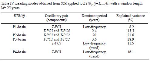
Now, we will analyze the time structure of evapotranspiration time series, ET(t)_j , (j=1, ...,4) derived from Eq. 3, for each sub–basin. SSA was applied to ET(t)_j time series(j=1, ...,4), with a window length M = 25 years, in order to detect signals, with a significance level greater than 95% (Allen and Smith, 1996).

4.1 P1–basin

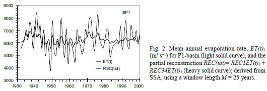
From the SSA applied to ET(t)₁ , we obtain that the first component, T–PC1, is associated with a low frequency signal, while the pair T–PC3 and T–PC4 is associated with a quasi–biennial oscillation, with period T ≈ 2.4 years. The period was obtained by computing the power spectrum of each principal component of the pair. The results are summarized in Table IV. Figure 2 shows the partial reconstruction for ET(t)_p based on T–EOF1 (REC1ET(t)₁), corresponding to the low frequency signal (accounting for 8.2% of the total variance); together with the reconstructed series based on the pair T–EOF3 and T–EOF4 (REC34ET(t)₁), corresponding to the quasi–biennial oscillatory mode (15.5%). These two signals are present in PR(t)₁ as it was shown by Krepper et al. (2008).

4.2 P2–Basin

The two leading components of ET(t)₂, T–PC1 and T–PC2, correspond to a significant quasi–oscillatory mode with period T ≈ 20 years, accounting for 21.6% of the total variance (see Table IV). According to Krepper et al., 2008, this signal was not present in PR(t)₂. These authors mentioned that PR(t)₂ is characterized by a small trend and periodicities in the ENSO–period range (2– to 5–years period). In fact, signals in the ENSO–period range are present in ET(t)₂, with low significance level. Therefore, the correlation between ET(t)₂ and PR(t)₂, previously mention, must be consequence of the shorter signals (in the ENSO–range) present in both time series. Each component of the hydrological cycle can introduce inherent signals to the system response. Figure 3 shows the partial reconstruction for ET(t)₂, based on the pair T–EOF1 and T–EOF2 (REC12ET(t)₂), corresponding to a bi–decadal oscillation.

4.3 P3–basin

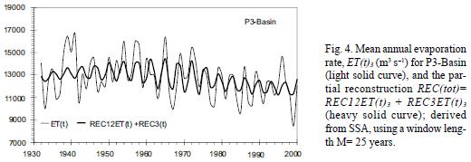
The results of applying a SSA to ET(t)₃ show two leading modes, T–PC1 and T–PC2, associated with an oscillatory component with dominant period T ≈ 3.6 years accounting for 29% of the total variance; and a low–frequency mode, T–PC3, associated to a negative trend after 1960 (11.5%). In this case, the ENSO–range signal (T ≈ 3.6 years) present in ET(t)₃ is also observed in PR(t)₃ (Krepper et al., 2008); while the negative trend (not present in PR(t)3) would indicate an impact of a land use change over the basin. Figure 4 shows the partial reconstruction for ET(t)₃, based on T–EOF1 (REC3ET(t)₃), corresponding to the low frequency signal; together with the reconstruction series based on the pair T–EOF1 and T–EOF2 (REC12ET(t)₃), corresponding to the oscillatory mode with T ≈ 3.6 years.

4.4 P4–Basin

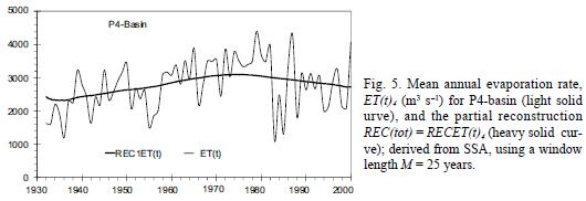
The P4–Basin presents a leading mode T–PC1 associated to a low–frequency signal, accounting for the 16.1% of the total variance (see Table IV). Figure 5 shows the partial reconstruction for ET(t)₄, based on T–EOF1 (RECET(t)₄), corresponding to the low frequency signal. PR(t)₄ does not presented this low frequency signal (Krepper et al., 2008). Then, the low–frequency behavior of ET(t)₄ must be caused by other factors, like changes in the lad–use or intrinsic basin properties.

 

5. Summary and discussion

The main objective of this paper was to analyze the structure of the ET time series of the upper Paraná basin. An annual water balance equation was applied at the sub–basin scale to obtain the time series ET(t) as a residual of the equation. We first studied the relationship between the variables in the water balance equation, then we applied a SSA to learn more about the temporal structure of the ET(t)_j time series.

From the analysis of mean annual contributions, , of each sub–basin, for 1931–1970 and 1971–2000 periods, we can observe that the drainage area upstream of Itaipú , and has increased the mean annual contribution after 1970 (see Table II). Meanwhile, remain quite constant(2590 m³s^–1 for 1931–1970 period and 2526 m³s^–1 after 1970). Table II also shows increases in and , from one period to other, especially for P3–basin where the change in is around 71%. The change in mean annual runoff response for P3–basin, could not be explained by an increasing in the corresponding mean annual precipitation rate, , because .

The evapotranspiration rates, obtained from a simplified balance given by Eq. 3 present a strong sub–basin dependence. Table IV shows the leading modes (significance level > 95%) obtained from SSA applied to ET(t)_j ( j = 1, ..., 4), using a ( T = 3.6 years) and a low–frequency signal window length M = 25 years. The time structure of ET(t)₁ time series (P1–basin) exhibits two significant modes, corresponding to a low–frequency signal and a quasi–biennial oscillation (T = 2.4 years), accounting for together around 24% of the total variance. The ET(t)₂ time series is dominated by a bi–decadal oscillation (T = 20 years) explaining 21.6% of variance. The southern sub–basins, ET(t)₃ and ET(t)₄ exhibit clear positive trends before 1970 and negative trends for the 1971–2000 period, accounting for 11.5 and 16.1% of variance, respectively. In the case ofthe ET(t)₃ time series, the low–frequency signal is accompanied by an interannual oscillation (T = 3.6 years) explaining 28.9% of variance. In other words, around 40% of the interannual variability, corresponding to ET(t)₃ time series, is explained by an ENSO–range period oscillation.

Looking at the whole basin, ET(t) would be affected either by changes in the basin physical properties or by the ENSO–range signal present in the precipitation. Other authors, i.e., Saurrall et al., (2008), suggested that the stream flow in the Uruguay river increased mainly due to the precipitation increase. They also suggested that the effects of land–used changes are negligible. On the contrary, Li et al. (2007) found that rainforest clear cut in Africa increased the annual streamflow in up to 65%. These examples of different studies show that there is not a simple unique response to climate and land–use change. In the case of La Plata Basin, every sub–basin would assimilate the land–use and climate changes through different mechanisms.

 

References

Allen R.M. and L. A. Smith, 1996. Monte Carlo SSA: Detecting irregular oscillations in presence of colored noise. Climate 9, 3373–3404.        [ Links ]

Anderson R.J., N. da Franca Ribbeiro dos Santos, and H.F. Diaz, 1993. An analysis of flooding in the Paraná/Paraguay River Basin. LATEN Dissemination Note # 5. The World Bank, Latin America & the Caribbean Technical Department, Environment Division.        [ Links ]

Berbery E.H., and V. R. Barros, 2002. The hydrologic cycle ofthe la Plata Basin in South America. J. Hydrometeorol. 3, 630–645.        [ Links ]

Brutsaert, W., 2005. Hydrology. An Introduction. Cambridge University Press, New York, USA, 605 pp.        [ Links ]

Carvalho L.M.V., C. Jones and B. Liebmann, 2004. The south Atlantic convergence zone: persistence, intensity, form, extreme precipitation and relationships with intraseasonal activity. J. Climate 17, 88–108.        [ Links ]

Castañeda M.E., and V. R. Barros, 1994. Las tendencias de la precipitación en el Cono Sur de América al este de los Andes. Meteorológica 19, 23–32.        [ Links ]

Comisión Mixta Paraguayo–Brasileña. 1974. Estudio del río Paraná: Informe final, factibilidad. Apéndice A: Hidrología y Meteorología. Andes–Electrobras, Asunción–Río de Janeiro, Brazil, 426 pp.        [ Links ]

Conway D., P. D. Jones, N. O. García, and W. M. Vargas, 1999. Assesing the Impact of Future Climatic Change on the Water Resources and Hydrology of the Rio de La Plata Basin, Argentina. Final Report of work under contract ARG/B7–3011/94/25a. Commision of European Communities; UK–Santa Fe: Argentina, 115 pp.        [ Links ]

Conway D., 2001. Understanding the hydrological impacts of land–cover and land–use change. IHDP Update Issue, 1, Article 2. Also available at http://www.ihdp.uni–bonn.de/html/publications/update/IHDPUdate01_,html. (Accesing: January, 2009).        [ Links ]

García N. O. and W. M. Vargas, 1996. The spatial variability of runoff and precipitation in the Rio de la Plata basin. Hydrolog. Sci. J. 41, 279–299.        [ Links ]

García N. O. and W.M. Vargas, 1998. The temporal climatic variability of runoff and precipitation in the Rio de la Plata basin. Climatic Change J. 38, 359–379.        [ Links ]

García N. O., 2000. Análisis de la variabilidad climática de la Cuenca del Río de la Plata, a través de los caudales de sus principales ríos. Ph. D. Thesis. Universidad Nacional de Córdoba, Argentina, 130 pp.        [ Links ]

Ghil M. and R. Vautard, 1991. Interdecadal oscillations and the warming trend in global temperature time series. Nature 350, 324–327.        [ Links ]

Ghil M., and P. Yiou, 1996. Spectral methods: What they can and cannot do for climatic time series. In: Decadal Climate Variability: Dynamics and Predictability, (D. Anderson and J. Willebrand, Eds.), Elsevier, Amsterdam, 446–482.        [ Links ]

Grimm A. M., S. E. T. Ferraz and J. Gomes, 1998. Precipitation anomalies in Southern Brazil associated wit El Niño and La Niña events. Climate 11, 2863–2880.        [ Links ]

Hulme M., 1994. Validation of large–scale precipitation fields in global circulation models. In: Global precipitations and climate changes. (M. Desbois and F. Desalmand, Eds.).Springer–Verlag, Berlín, 466 pp.        [ Links ]

Jothiyangkoo C., M..Sivapalan and D. L. Farmer, 2001. Process controls of water balance variability in a large semi–arid catchment: downward approach to hydrological model development. J. Hydrol. 254, 174–198.        [ Links ]

Krepper C.M., and M. E. Sequeira, 1998. Low frequency variability of rainfall in Southeastern South America. Theor. Appl. Climatology 61, 19–28.        [ Links ]

Krepper C. M., N. O. Garcia, P. D. Jones, 2008. Low–frequency response of the upper Paraná basin. Int. J. Climatol. 28, 351–360.        [ Links ]

Le Breton R. J. G., 1998. Sustainable land use in the Atlantic rainforest of Brazil. Iracambi Atlantica Rainforest Research and Conservation Center, Iracambi, Brazil, 20. Also available at http://www.iracambi.com.        [ Links ]

Li K. Y., M. T. Coe, N. Ramankutty and R. de Jong, 2007. Modeling the hydrological impact of land–use change in west Africa. J. Hydrol. 337, 258–268.        [ Links ]

Manabe S., 1969. Climate and the ocean circulation. II The atmospheric circulation and the effect of heat transfer by ocean currents. Mon. Weather Rev. 97, 775–805.        [ Links ]

Marengo J. A. and C. C. Camargo, 2007. Surface air temperature trends in southern Brazil for 1960–2002. Int. J. Climatol. 28, 893–904.        [ Links ]

Milly, P. C. D., 1994. Climate, soil water storage, and the average annual water balance. Water Resour. Res. 30, 2143–2156.        [ Links ]

Minetti J. L., and W. M. Vargas, 1998. Trends and jumps in the annual precipitation in South America, south of 15° S. Atmósfera 11, 205–221.        [ Links ]

Mitchell T. D., T. R. Carter, P. D. Jones, M. Hulme and M. New, 2004. A comprehensive set of high–resolution grids of monthly climate for Europe and the globe: the observed record (1921–2000) and 16 scenarios (2001–2010). Tyndal Centre Working Paper, 55, 25 pp.        [ Links ]

Mitchell T. D. and P. D. Jones, 2005. An improved methods of constructing a data base of monthly climate observations and associated high–resolution grids. Int. J. Climatol. 25, 693–712.        [ Links ]

New M., M. Hulme and P. D. Jones, 2000. Representing twentieth century space–time climate variability. Part 2: development of 1901 –96 monthly grids of terrestrial surface climate. Climate 13, 2217–2238.        [ Links ]

Plaut G. and R. Vautard, 1994. Spells of low–frequency oscillation and weather regimes in the Northern Hemisphere. J. Atmos. Sci. 51, 210–236.        [ Links ]

Saurral R. I., V. R. Barros and D. P. Lettenmaier, 2008. Land use impact on the Uruguay River discharge. Geophys. Res. Lett. 35, L12401, doi: 10.1029/2008GL033707.        [ Links ]

Schnepf R. D., E. Dohlman and C. Bolling, 2001. Agricultural in Brazil and Argentina: Developments and prospects for maj or field crops. ERS Agriculture and Trade Report No. WRSO13; 85.        [ Links ]

Sokolov A. A. and T. G. Chapman, 1974. Methods for water balance computations. The UNESCO Press. Paris, France. 127 pp.        [ Links ]

Tucci C. E. M. and R. T. Clarke, 1998. Environmental issues in the la Plata Basin. Int. J. Water Resour. D. 14, 157–173.        [ Links ]

Vautard R. and M. Ghil, 1989. Singular spectrum analysis in non–linear dynamics with applications to paleoclimatic time series. Physica D 35, 395–424.        [ Links ]

Vera C.S., P.K. Vigliarolo and E. H. Berbery, 2002. Cold season synoptic scale waves over subtropical South America. Mon. Weather Rev. 130, 684–699.        [ Links ]

Wang G. and E. A. B. Eltahir, 2000. Role of vegetation dynamics in enhancing the low–frequency variability of the Sahel rainfall. Water Resour. Res. 36, 1013–1021.        [ Links ]