


Services on Demand
Journal

Article
 English (pdf)
 Article in xml format
 Article references
 Send this article by e-mail
Indicators
 Cited by SciELO
 Related links
-
 Similars in
SciELO
Similars in
SciELO
Share

 Permalink
Atmósfera
Print version ISSN 0187-6236
Atmósfera vol.22 n.3 Ciudad de México Jul. 2009
An approach to seasonal forecasting of summer rainfall in Buenos Aires, Argentina
M. H. GONZÁLEZ
Departamento de Ciencias de la Atmósfera y los Océanos,
Facultad de Ciencias Exactas y Naturales, Universidad de Buenos Aires
Ciudad Autónoma de Buenos Aires, Argentina.
Corresponding author; e–mail: gonzalez@cima.fcen.uba.ar
M. L. CARIAGA
Centro de Investigaciones del Mar y la Atmósfera, Consejo Nacional de Investigaciones
Científicas y Tecnológicas, Universidad de Buenos Aires, Argentina.
Received August 18, 2008; Accepted March 30, 2009
RESUMEN
Este trabajo presenta algunas características de la precipitación estival y un modelo de predicción estacional en la región metropolitana de Buenos Aires. La ciudad de Buenos Aires está ubicada en la costa del Río de la Plata en Argentina. El rasgo principal de la precipitación es un ciclo anual con máximo en la época de verano. La tendencia de precipitación anual observada desde 1908 fue de 2.1 mm/año mientras que para la lluvia estival fue de 1.8 mm/año. La estación Observatorio Central Buenos Aires, ubicada en el centro de la ciudad, registró una precipitación anual acumulada media durante el período 1908–2007 de 1070 mm con un desvío standard de 239 mm. Durante los meses de diciembre, enero y febrero se acumuló en forma media un total de 305 mm con desvío de 125 mm. La identificación de períodos húmedos y secos permitió concluir que los períodos secos tendieron a ocurrir con mayor frecuencia en 1908–1957 mientras que los húmedos fueron más intensos y frecuentes en 1958–2007. La lluvia acumulada entre diciembre y febrero fue relacionada con los campos medios de algunas variables meteorológicas entre septiembre y noviembre, con el fin de desarrollar un modelo de predicción. Los predictores fueron cuidadosamente elegidos basándose especialmente en su interpretación física. El modelo de regresión fue derivado utilizando la metodología conocida como forward stepwise. Los resultados mostraron que la mayor fuente de predictabilidad se encontró en la actividad ciclónica del Océano Atlántico próximo al continente y en el flujo de aire desde la selva brasileña. La precipitación observada y la pronosticada estuvieron significativamente correlacionadas (0.59) y el modelo explicó el 35% de la varianza de la lluvia estival. Se realizó la validación semi–cuantitativa, calculando los terciles de las distribuciones de lluvia observada y pronosticada. Los resultados fueron satisfactorios aunque una porción de la varianza no ha sido explicada por el modelo y la eficiencia del mismo podría ser mejorada en futuros trabajos.
ABSTRACT
This paper analyzes some summer rainfall characteristics in Buenos Aires and developes a seasonal prediction scheme. Buenos Aires is located along the coast of the Río de la Plata in Argentina. The outstanding rainfall feature is the presence of an annual cycle with maximum precipitation in summer. The analysis of the annual rainfall evolution since 1908 showed a positive trend of 2.1 mm/year and 1.8 mm/year for the period between December and February, representative of the summer season. The Observatorio Central Buenos Aires/station, located in the downtown, registered a mean annual accumulated rainfall of 1070 mm with a standard deviation of 239 mm, during the period 1908–2007. The mean accumulated precipitation during January, February and March was 305 mm with a standard deviation of 125 mm. The wet and dry periods were identified and the dry periods tended to be longer during 1908–1957 meanwhile wet periods resulted longer and more intense in 1958–2007. Accumulated rainfall between December and February was related to some mean meteorological variables between September and November, with the aim to develop a statistical prediction scheme. Careful selection of predictors, based largely on physical reasoning, was done and they were used in a regression model, following a forward stepwise methodology. The analysis shows that the most important source of predictability comes from the cyclonic activity in the Atlantic Ocean and the flow from Brazilian forest. The observed and forecast rainfall series were significantly correlated (0.59) and nearly the 35% of summer rainfall variance was predicted by the proposed method. A semi–quantitative validation was done by using terciles of the observed and forecast distributions. The skill of the forecast got a good result although there is still an important portion of the variance that cannot be explained by this model and therefore, the method might be improved in future research.
Keywords: Rainfall, statistical prediction model, sea surface temperature, pattern circulation, standarized precipitation index.
1. Introduction
Argentina is located in the southeastern part of South America and occupies a total area of 2,791,810 km2. Because of its large extension, areas with different climate features can be described. West to South America, the Andes Mountain range is one of the main features which has great influence on the climate of the region. It is the most important mountain range in America and one of the most relevant in the world. It is bordered by highlands or separated from other mountains by passes and valleys. It is 7240 km long and crosses Venezuela, Colombia, Ecuador, Bolivia, Chile and Argentina, all along the western coast of South America. It is 200 to 700 km wide and it has a mean height of 3660 m although some peaks reach more than 6000 m. The highest peak, Aconcagua, rises to 6962 m above sea level and it is located in Argentina. Two regions can be distinguished in Argentina: the first, north of 38°S is high and solid meanwhile the southern sector is lower and less dense. Therefore, north of 38°S, the Andes range prevents the access of humidity from the Pacific Ocean, the flow is governed by the South Atlantic Height and as a consequence, winds prevail from the northeast. Therefore, the water vapor entering at low levels comes either from the tropical continent or from the Atlantic Ocean. In the first case, the easterly low–level flow at low latitudes is channeled towards the south between the Bolivian Plateau and the Brazilian forest, advecting warm and humid air to southern Brazil, Paraguay, Uruguay and subtropical Argentina and depicting a typical feature that many authors have studied (Lenters and Cook, 1995; Wang and Paegle, 1996; Barros et al., 2002; Vera et al., 2006). Intermittent eruptions of polar fronts from the south modify this picture, causing a west or a southwest flow in low levels after the frontal passage. This happens with more frequency and greater displacement to the north in winter than in summer. González and Barros (1998) analyzed the mean annual rainfall cycle in subtropical Argentina using a principal component analysis and showed a minimum in winter, which is more pronounced in the west, with dry conditions prevailing from May to September and a region in central Argentina where rainfall had two peaks, both in transition seasons. That is the case in Buenos Aires city and the surrounding areas, located along the coast of the Río de la Plata, over the coast of the Atlantic Ocean. This area has experienced a great urban center and population growth and so it conjugates the problematic of the natural rainfall variability and the influence of human activity on it.
Therefore, some researchers have detected changes on the behavior of annual rainfall. For example, Castañeda and Barros (1994) detected a considerable increase in precipitation from the 60s in most of the Argentine territory, especially during summer (Barros and Castañeda, 2001).
The surrounding areas of the city are well known because of the fruit and vegetable productions where precipitation is a necessary resource for such productions in small farms generally run by individuals. Seasonal rainfall forecast is relevant for planning such economic activities. Seasonal climate predictability has its scientist basis in the fact that slow variations in the earth's boundary conditions (i.e. sea surface temperature or soil wetness), can influence global atmospheric circulation and thus precipitation. As the skill of seasonal numerical prediction models is still very limited, it is essential the statistical study of the probable relationships between some local or remote forcing and rainfall in each place and season. Some authors have explored techniques with the aim of forecasting seasonal rainfall in different areas in the southern hemisphere. For example, Zheng and Frederiksen (2006) explained 20% (17%) for summer (winter) rainfall in Australia using a regression model with sea surface temperature (SST) predictors, after removing the intraseasonal variability. Gissila et al. (2004) used a regression model to predict Ethiopian rainfall in rainy season, using some SST predictors and Reason (2001) did it for South Africa. Singhrattna et al. (2005) develop two methods, a linear regression and a polynomial–based non parametric, for forecasting Thailand summer monsoon rainfall. They made a significant contribution because although both methods exhibit significant skill, the second one was more efficient specially during extreme wet and dry years.
This paper intends to contribute to the knowledge of rainfall behavior and explore local and general circulation patterns, which can explain summer rainfall anomalies in Buenos Aires. It is organized as follows: Section 2 describes the Dataset; Section 3 the Methodology; and Section 4 the Results. Section 4.1 analyses the General Rainfall Features and its evolution in the last century and Section 4.2 deals with the relationship between summer rainfall variability and regional circulation patterns. Finally, in Section 4.3, a statistical prediction model is developed to forecast summer rainfall in the Buenos Aires area.
2. Data
Monthly rainfall data for the period 1908 to 2007 in Observatorio Central Buenos Aires station (OCBA) –that belongs to the Servicio Meteorológico Nacional network– was used to analyze the characteristics of rainfall. This series has no missing data.
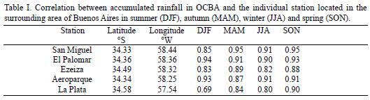
Some other stations from this network (San Miguel, El Palomar, Ezeiza, Aeroparque and La Plata, see Table I for location), located in the surrounding of OCBA, were used to study the relationship between summer rainfall and some circulation patterns in the period 1959–2007. This period was used because all the stations have less than 5% of missing monthly rainfall data, except for La Plata, which has 8% missing data.
Monthly SST, 500 Hpa and 1000 Hpa geopotential heights (500GH, 1000GH), 850 Hpa zonal (85U) and meridional (85V) wind, and sea level pressure (SLP) from National Center of Environmental Prediction (NCEP) reanalysis were used to study the regional and hemispheric patterns during 1959–2007 (Kalnay et al., 1996).
The predictors selected to develop the model were: the SST along the Brazilian coast between 10° and 15°S, the SST in the South Pacific Ocean, between 40° and 45°S, west of Chile, SLP in the Atlantic Ocean centered in 30°S and 30°W, and 85U averaged in an area located around 20°S over central South America. All these variables were averaged from September to November.
3. Methodology
The mean monthly evolution of rainfall in OCBA was evaluated. The annual and summer (December to February, DJF hereinafter; all 3–months periods will be similarly abbreviated) precipitation trend in OCBA were computed and their significance evaluated using the Mann Kendall (Mann, 1945) test. It is a non–parametric test for detection of trend; it does not assume any particular distribution of the data and compares each value with all the values measured in subsequent periods.
The standardized precipitation index (SPI) was used to assess the conditions of deficit or excess of precipitation, for three months time interval (McKee et al., 1993, 1995), with the purpose of improving the detection of rainfall excesses and deficits which could produce significant consequences in the farming production. Computation of the SPI involves fitting a gamma probability density function to a given frequency distribution of precipitation totals for OCBA. The parameters of the gamma distribution are estimated for the station, for the time scale of interest (3 months in this case), and for each month of the year. The cumulative probability according to the distribution, and for each value of precipitation, is transformed to the standard normal random variable Z with a mean of zero and a variance of one, which is the value of the SPI. According to McKee et al. (1993), the index has a normal distribution, so it can be used to estimate both dry and wet periods. According to the SPI, a wet (dry) period is defined as the period during which the SPI is continuously positive (negative).
The magnitude of the index allows classifying the three month accumulated rainfall in categories that go from extreme drought to extreme excess (extremely dry, severe dry, moderate dry, normal, moderate wet, severe wet and extremely wet) (Mckee et al., 1993).
A mean rainfall series (AMBA) was constructed as the average of monthly precipitation of six stations in the area of study, with the aim of being representative from the area at issue for the period 1959–2007, when all the stations had complete records. As it can be observed in Table I, the high correlations between three months accumulated rainfall in each one of the individual stations and OCBA, are all significant at 95% confidence level.
Simultaneous and three months lagged correlations were calculated to find the existing relation between summer rainfall and sea surface temperature. As the precipitation process is directly related not only to the water vapor content but also to pressure systems that provide the necessary ascent mechanisms, the relationships between rainfall and 1000 Hpa, 500 Hpa geopotential height and SLP are analyzed too.
The results allowed defining some predictors (SST in the Atlantic Ocean, along the Brazilian coast, SST in the Pacific Ocean, west of Chile, SLP in the Atlantic Ocean and 85U around 20°S in South America), which were used for developing a statistical forecast model for summer rainfall in AMBA. This model was derived using the forward stepwise regression method (Wilks, 1995).
4. Results and discussion
4.1 General rainfall features
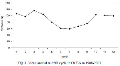
Despite the fact it rains all along the year, this area is characterized by summer rainfall as it can be observed in the mean monthly precipitation for 1908–2007 period in OCBA (Fig. 1) and this is the reason why this paper will mainly deal with the period DJF, representative of summer rainfall.
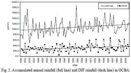
Until now, linear trend approximation has been the simplest way to evaluate the observed change in a time series (Panofsky and Brier, 1965; Darlington, 1990; Wilks, 1995). This approach can represent precipitation time evolution efficiently in a given period. Figure 2 shows annual and DJF rainfall linear trends in OCBA, calculated with observed data registered during 1908–2007 period. Increments of 2.1 mm/year and 1.8 mm/year were registered for the annual and DJF cases, respectively, as Castañeda and Barros (2001) have already pointed out for a shorter period.
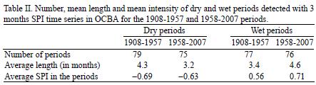
By using the 3–month SPI, well–defined wet and dry cycles are identified in OCBA from the time series analyzed. The results were detailed in Table II, distinguishing two main periods: the first fifty years 1908–1957 and the last ones 1958–2007, with the aim to detect differences between them. Although the number of wet and dry periods in both stages was similar, dry periods tended to be longer in 1908–1957 meanwhile wet periods resulted longer and more intense in 1958–2007. Therefore, the 25.3% of the dry periods resulted moderate to extreme in 1908–1957 but only the 14.6% in 1958–2007. In addition, the 11.7% of the wet periods were of moderate to extreme intensity in 1908–1957, meanwhile this percentage increase to 30.3% in 1958–2007. Penalba and Vargas (1996) have found similar results and they pointed out that the driest periods in Buenos Aires plains generally prevail before 1940 meanwhile wet periods are well distributed all along the last century.
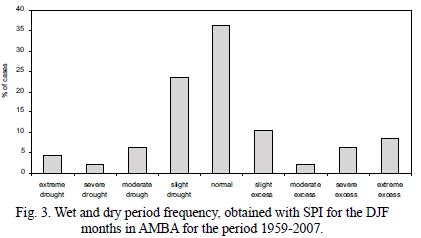
A similar analysis was performed for the AMBA time series for the period 1959–2007. Figure 3 shows the wet and dry periods frequency, as defined with SPI for the DJF months. Almost 10% of the years have been classified as extreme excess (1977, 1984, 1990, 2003) and severe excess (1971, 1998, 1999) meanwhile 7% of the years approximately detected extreme (1960, 1979, 1989) and severe (1968) droughts in DJF.
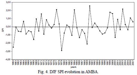
The DJF SPI evolution (Fig. 4) showed an important interannual variability and a slight trend to larger SPI values.
4.2 Relation between summer rainfall in AMBA and SST, low and middle level flow and sea level pressure patterns
In this section a seasonal forecasting model for the Buenos Aires region using a simple regression model will be developed. The first stage of the model is to determine statistical associations between rainfall and circulation patterns. There are evidences that rainfall patterns in the study region are related to remote forcing. The most important is probably the El Niño–Southern Oscillation (ENSO) phenomenon, which was largely studied by many authors in the Argentinean region (e. g. Grimm et al., 2000). However, the presence of other remote forcing must be considered, for example Zheng and Frederiksen (2006) demonstrated that SST conditions in central Indian Ocean in MAM are a good predictor of winter rainfall variability in New Zealand. Reason (2001) and Gissila (2004) described links between Indian Ocean SST variability and rainfall in South Africa and Ethiopia, respectively. Singhrattna et al. (2005) found a clear relation between SLP in the Pacific subtropical ocean and SST in the Indian Ocean with the Thailand summer monsoon rainfall. However, there are no studies which show the link between Indian Ocean SST and rainfall in extra–tropical South America. In many cases, the relationship to remote forcing can increase the chances of success of seasonal predictability because it can be extended out to longer ranges based on the influences of slowly evolving boundary conditions on the atmospheric circulation, such as the sea surface temperature or the soil wetness and, hence, seasonal climate can tilt in a specific direction. For example, in the subtropical latitudes of South America, the Andes Mountains block the low–level flow between the eastern Pacific and South America and thus SST anomalies in the western and central Pacific appear to have influence on south American rainfall through Rossby wave propagation (Kalnay et al., 1986). Hence, considering these relationships and that SST anomalies generally undergo slow changes in the intra–seasonal scale, they are explored as possible predictors of rainfall in the study area.
Therefore, AMBA accumulated precipitation time series during DJF, over the 1959–2007 period was associated to SST, 500GH, 1000GH, 85U, 85V and SLP fields and highlighted areas of importance for predicting rainfall were detected. The correlation was calculated for the simultaneous period and for one (NDJ), two (OND) and three (SON) months before the DJF rainfall.
The statistical associations between rainfall and the previous variables were assessed by calculating lineal correlation between DJF rainfall and the spatial field of the different variables (SST, 500GH, 1000GH, 85U, 85V and SLP) for 49 years, and so the correlation required for significance at 95% level was 0.28.
Figure 5 shows the correlation between DJF rainfall in AMBA and SON (Fig. 5a), OND (Fig. 5b), NDJ (Fig. 5c) and DJF SST (Fig. 5d). There are areas where SST exhibit significant lagged correlation with AMBA rainfall. The main regions with significant correlation with SON SST (Fig. 5a) are located in the tropical Pacific (130–90°W and 0–10°S) (A1), along the Brazilian coast between 10 and 15°S (A2), and in the south Pacific Ocean, between 40 and 45°S, west of Chile (A3). A1 indicates the tendency to rainiest summer when a warm event was present; A2 depicts the enhanced evaporation in warm water (25.6°C which increases to 26.7°C approximately in the warmest cases) in an area where the Atlantic Height causes the entrance of humid air into the continent, and so water vapor enriched the flow from the north in Buenos Aires. The negative correlation in A3 is probably associated with the modified trajectories of cyclonic systems and fronts, which produce rainfall as they arrive to Buenos Aires from the south. These main regions associated with DJF rainfall are noticeable in OND, NDJ and DJF, although with less values (Fig. 5b, 5c and 5d).
The same analysis was performed on 500GH and 1000GH. Only the correlation fields between SON geopotential heights and DJF rainfall are shown in this paper. An area with strong negative association centered in 30 and 30°W in the south Atlantic Ocean (A4), is depicted in 1000GH case (Fig. 6), meanwhile a zonal extended area from the Atlantic to the Pacific Oceans, located around 25°S (A5) is the main feature in 500GH field (Fig. 7). In both cases, they indicate that the presence of low–pressure systems enhances the possibility of precipitation in Buenos Aires. The same physical effect can be detected in the correlation fields between SON SLP and DJF rainfall in AMBA (Fig. 8), where a significant negative correlation center is positioned in the Atlantic Ocean (A6), as in the case of 1000GH .
Low–level flow was also analyzed in order to evaluate the water vapor advection. Correlation between SON 85U and DJF rainfall in AMBA (Fig. 9) shows a dipole formed by an elongated zone of positive values, located around 20°S over central South America (A7) and a center of negative correlation northern of the previous mentioned, around 15°S (A8). This pattern indicates that the entrance of humid air from the Atlantic Ocean near 15°S favored DJF rainfall in Buenos Aires. Then the Andes Mountains channel the flow towards the south and it rotates to the east near 20°S.
The previous detailed effect is also visible when DJF rainfall in AMBA is correlated with 85V (Fig. 10) and a negative correlation center is present around 15°S–65°W (A9), indicating that rainfall is favored by the northern flow. Besides, a positive one is located near 30°S–62°W (A10), probably associated to the southern flow related to frontal systems.
4.3 The prediction model
In order to select the best predictors for the model, boxes from A1 to A10, as defined in the above section and in the respective figures, were used to calculate the linear correlation between the mean SON variable in the box and the DJF rainfall in AMBA (Table III).
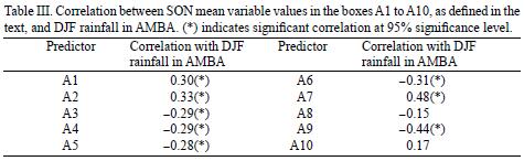
Predictors available to carry out the regression scheme were carefully selected, based on statistical significance and physical reasoning. The choice of input variables for the regression model was done between the predictors described in Table III. Only the predictors with correlation greater than 0.28 were considered. However, as they must be independent among each other, A1, A4 and A9 were rejected because they had significant correlation with some of the others. Finally, the input predictors for the model were A2, A3, A6 and A7. The selected model was a forward stepwise regression, which retained only the variables, correlated with 95% significance level. Forward stepwise regression is a model–building technique that finds subsets of predictor variables that most adequately predict responses on a dependent variable by linear regression, given the specified criteria for adequacy of model fit (Darlington, 1990). The basic procedures involve identifying an initial model, repeatedly altering the model at the previous step by adding a predictor variable in accordance with a fixed criterion, and terminating the search when stepping is no longer possible according to the criteria.
The approach used in this paper was to split into two subsets (Farmer, 1988). The training period 1959–1983 was used to develop the model and the 1984–2007 for verification. The derived model was:
P = –32.6 A6 + 74.8 A7 + 33456.2
P is the predicted accumulated rainfall in DJF for AMBA. The percentage of variance explained by the model was 35% with a linear regression coefficient of 0.59. A commonly used measure of strength of the regression is the F–ratio, defined as the relationship between the mean square regression and the mean square error (Wilks, 1995). It is desirable that the F–ratio was high because a strong relationship between P and the predictors will produce large mean square regression and small mean square error. As the residual of the regression is independent and follow a normal distribution, under the null hypothesis of no linear regression, the F–ratio was 5.6 with a p–value of 0.01, and therefore, the regression model provides reasonably forecast with 95% of confidence.
The method only retained the predictors A6 and A7 from the four candidate predictors, indicating that the two major factors that influence summer precipitation in that area are: the SLP in the Atlantic coast and low–level flow from Brazilian forest. This result enhanced the importance of northern flow in summer in the region of study. Summer circulation consists of an easterly flow from the tropical Atlantic Ocean height. This flow turns to the south after reaching the proximity of the Andes and is channeled towards the south across the Brazilian forest, advecting humid air to the southern part of the continent. It could be one of the links between the Amazon convection and subtropical rainfall (González and Barros, 1998).
Validation is an important component of the model construction, a recommendable method is to construct the model with a subset of the available data and then test the model over the remaining period (Wilks, 1995). Unfortunately, this approach reduced the number of observations available to train the model. In this case, the verification was done for the period 1984–2007 and the predicted and observed series were significant correlated (0.54) at the 95% confidence level (Fig. 11).
Other sets of predictors were proved as input variables for the model and the same ones were selected by the method, indicating that there was no evidence of numerical instability.
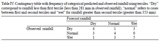
The skill of the forecast has been measured in semi–quantitative terms as follows: the observed rainfall distribution in the period 1984–2007 was categorized in terciles and the same was done for the forecasted rainfall distribution. The observed and predicted rainfall terciles, were then compared by constructing a contingency table (Table IV). This contingency table differs significantly from a random one at 80% confidence level, using a Chi–square test.
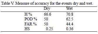
The most direct and intuitive measure of the accuracy of the categorized forecast (Wilks, 1995) is the hit rate (H) or the right proportion. It is the fraction of all the cases when the categorical forecast correctly anticipated the subsequent event. The probability of detection (POD) is defined as the fraction of those occasions when the forecasted event occurred on which it was also forecast. The false alarm relation (FAR) is the proportion of forecast events that fail to happen. The Heidke score (HS) is a relative accuracy measure that compares the skill of the forecast with the hit rate that would be achieved by random forecast. The perfect forecast receives Heidke score of one, forecasts equivalent to reference forecast (random) receive score zero and negative values imply that the forecast are worse than the reference one.
Table V shows these accuracy measures for the events "dry" and "wet". They are calculated collapsing the 3 x 3 contingency table into two 2 x 2 tables. Each one is constructed by considering the "forecast event" (dry or wet) as opposed to the complementary "non forecast event" (non–dry or non–wet). The values in Table V indicate that the method detects some cases of extreme rainfall, improving the random forecast (as the Heidke scores indicate) but it must be improved for better results.
5. Conclusions
The area of Buenos Aires is characterized by summer rainfall. During the1908–2007 period, a positive trend of 2.1 mm/year and 1.8 mm/year were registered for the annual and DJF cases respectively in OCBA. An analysis of SPI demonstrated that although the number of wet and dry periods in both stages, 1908–1957 and 1958–2007, were similar, dry periods tended to be longer in the first one meanwhile wet periods resulted longer and more intense in the last.
In order to develop a statistical prediction scheme for DJF rainfall, a mean areal rainfall series, called AMBA, was defined as the average of monthly precipitation of six stations in the area of study. AMBA rainfall was correlated with sea surface temperature, sea level pressure, geopotential height and low–level winds observed three months before, to identify predictors, which can be used in a regression model. A forward stepwise methodology was used and a prediction model was developed for the period 1959–1983. The analysis shows that the most important source of predictability comes from the cyclonic activity in the Atlantic coast and the flow from Brazilian forest, both used as predictors in the prediction scheme. The observed and forecast rainfall series for the validation period (1984–2007) were significantly correlated (0.59). Although, nearly the 35% of summer rainfall variance is predicted by the proposed method, there is still an important portion of the variance that cannot be predicted by it. In the future, it will be desirable to improve the skill of the method.
Acknowledgements
Rainfall data were provided by the Servicio Meteorológico Nacional. Images from figures 5 to 10 (figures 5, 6, 7, 8, 9 and 10) were provided by the NOAA/ESRL Physical Sciences Division, Boulder CO from their web site: http:www–cdc–noaa–gov. This research was supported by UBACyT X444, UBACyT X160 and CONICET PIP 112–200801–00195.
References
Barros V. R. and M. E. Castañeda, 2001. Tendencias de la precipitación en el oeste de Argentina. Meteorologica 26, 5–24. [ Links ]
Barros V., M. Doyle, M. H. González, I. Camilloni, R. Bejarán and M. Caffera, 2002. Revision of the south American monsoon system and climate in subtropical South America south of 20°S. Meteorologica 27, 33–58. [ Links ]
Castañeda M. E. and V. Barros, 1994. Las tendencias de la precipitación en el Cono Sur de América al este de los Andes. Meteorologica 19, 23–32. [ Links ]
Darlington R. B., 1990. Regression and linear models. McGraw–Hill. New York, 542 pp. [ Links ]
Farmer G., 1988. Seasonal forecasting of the Kenya coast short rains 1901–1984. Int. J. Climatol. 8, 489–497. [ Links ]
Gissila T., E. Black, D. I. F. Grime and J. M. Slingo, 2004. Seasonal forecasting of the Ethiopian summer rains. Int. J. Climatol. 24, 1345–1358. [ Links ]
González M. H. and V. Barros, 1998. The relation between tropical convection in South America and the end of the dry period in subtropical Argentina. Int. J. Climatol. 18, 1669–1685. [ Links ]
Grimm A., V. Barros and M. Doyle, 2000. Climate variability in southern South America associated with El Niño and La Niña events. J. Climate 13, 35–58. [ Links ]
Kalnay E., K. C. Mo and J. Paegle, 1986. Large–amplitude, short scale stationary Rossby waves in the Southern Hemisphere: Observations and mechanistics experiments on determine their origin. J. Atmos. Sci. 3, 252–275. [ Links ]
Kalnay E., M. Kanamitsu, R. Kistler, W. Collins, D. Deaven, L. Gandin, M. Iredell, S. Saha, G. White, J. Woollen, I. Zhu, M. Chelliah, W. Ebisuzaki, W. Higgings, J. Janowiak, K.C. Mo, C. Ropelewski, J. Wang, A. Leetmaa, R. Reynolds, R. Jenne and D. Joseph, 1996. The NCEP/NCAR Reanalysis 40 years– project. Bull. Amer. Meteor. Soc. 77, 437–471. [ Links ]
Lenters J. D and K. H. Cook, 1997. On the origin of Bolivian high and related circulation feature of the South American climate J. Atmos. Sci. 54, 656–677. [ Links ]
Mann H. B., 1945. Non–parametric tests against trend. Econometrica 13, 245–259. [ Links ]
McKee T., N. Doesken and J. Kleist, 1993. The relationship of drought frequency and duration to times scales. 8th Conference of Applied Climatology, Anaheim, CA, USA, January 1993, 179–184. [ Links ]
McKee T. B, N. Doesken and J. Kleist, 1995. Drought monitoring with multiple time scales. Ninth Conference on Applied Climatology, Dallas, TX, USA, January 1995, 233–236. [ Links ]
Panofsky H. A. and G. W. Brier, 1965. Some applications of statistics to meteorology. Mineral Industries Continuing Education, College of Mineral Industries, The Pennsylvania State University. University Park, Pennsylvania, 224 pp. [ Links ]
Penalba O. C. and M. W. Vargas, 1996. Climatology of monthly and annual rainfall in Buenos Aires, Argentina. Meteorol. Appl. 3, 275–282. [ Links ]
Reason C., 2001. Subtropical Indian Ocean SST dipole events and Southern Africa rainfall. Geophys. Res. Lett. 28, 2225–2227. [ Links ]
Singhrattna N., B. Rajagopalan, M. Clark and K. Krishna Kumar. 2005. Seasonal forecasting of Thailand summer monsoon rainfall. Int. Climatol. 25, 649–664. [ Links ]
Vera C., W. Higgins, J. Amador, T. Ambrizzi, R. Garreaud, D. Gochis, D. Gutzler, D. Lettenmaier, J. Marengo, C. R. Mechoso, J. Nogues–Paegle, P. L. Silva Dias, and C. Zhang, 2006. Toward a unified view of the American Monsoon Systems. J. Climate 19, 4977–5000. [ Links ]
Wang M. and J. Paegle, 1996. Impact of analysis uncertainty upon regional atmospheric moisture flux. J. Geophys. Res. 101, 7291–7303. [ Links ]
Wilks D. S., 1995. Statistical methods in the atmospheric sciences (An introduction). International Geophysics Series. Academic Press, San Diego, CA, USA, 467 pp. [ Links ]
Zheng X. and C. Frederiksen, 2006. A study of predictable patterns for seasonal forecasting of New Zealand rainfall. J. Climate 19, 3320–3333. [ Links ]
Zhou J. and K. M. Lau, 1998. Does a monsoon climate exist over South America? J. Climate 11, 1020–1040. [ Links ]

