Bivariate distribution with two–component extreme value marginals to model extreme wind speeds

 

C. ESCALANTE–SANDOVAL
División de Ingenierías Civil y Geomática, Facultad de Ingeniería,
Universidad Nacional Autónoma de México, 04510 México, D. F., México
E–mail: caes@servidor.unam.mx

 

Received June 7, 2007; accepted June 9, 2008

 

RESUMEN

Se aplica el modelo logístico bivariado con distribuciones marginales de valores extremos de dos componentes (BTCEV) para obtener un estimador regional de las velocidades de viento. Los parámetros fueron calculados por el método de máxima verosimilitud a través de un algoritmo de optimización multivariado restringido. El modelo se ajustó a los registros de velocidades de vientos extremos de 45 estaciones localizadas en Holanda. Los resultados fueron comparados con aquellos obtenidos por el ajuste de las distribuciones Gumbel (G), General de Valores Extremos (GVE), Weibull Inversa (RW) y valores exremos de dos componentes (TCEV); las distribuciones bivariadas con marginales G, GVE y RW y tres métodos regionales: estaciones–año, avenida índice (viento–índice) y momentos–L. En general, se tienen mejoras significativas, medidas a través de un criterio de bondad de ajuste, empleando la modelación bivariada en comparación de su contraparte univariada y regional, y las diferencias entre los estimadores en el sitio y regional de los eventos de diseño pueden ser importantes conforme se incrementa el periodo de retorno. Los resultados sugieren que es muy importante considerar el uso de las distribuciones bivariadas para el ajuste de velocidades de viento extremo, especialmente para el caso de muestras pequeñas.

 

ABSTRACT

The bivariate logistic model with two–component extreme value marginal distributions (BTCEV) is applied to provide a regional at–site wind speed estimate. The maximum likelihood estimators of the parameters were obtained numerically by using a multivariable constrained optimization algorithm. A total of 45 sets of largest annual wind speeds gathered of stations located in The Netherlands were selected to apply the model. Results were compared with those obtained by the univariate distributions: Gumbel (G), Generalized Extreme Value (GEV), Reverse Weibull (RW) and two–component extreme value (TCEV); the bivariate distributions with marginals G, GEV and RW; and three regional methods: station–year, index flood (index–wind) and L–moments. In general, a significant improvement occurs, measured through the use of a goodness–of–fit test, when estimating the parameters of the marginal distribution with the bivariate distributions instead of its univariate and regional counterpart, and differences between at–site and regional at–site design events can be significant as return period increases. Results suggest that it is very important to consider the bivariate joint estimation option when analyzing extreme wind speeds, especially for short samples.

Keywords: Wind speed frequency analysis, bivariate extreme value distribution, maximum likelihood parameter estimation, goodness–of–fit.

 

1. Introduction

Extreme wind speeds (EWS) have been analyzed through the use of univariate distributions. Several assumptions underlay the statistical estimate of the wind speed. The most important one, that all extremes (up to return periods of 10⁴ yr) belong to the same population, is hard to verify from the available short observational sets.

Van Den Brink et al. (2004) noticed the existence of areas where the extreme value distribution of extratropical winds was double populated. They demonstrated that the local wind can be caused by two meteorological systems a and b of different physical nature, each of them generating its own distribution F_a(s) and F_b(s). Then, the parent distribution F(s) is said to be mixed. The simplest case of F(s) represents the multiplication of two exponential distributions which Rossi et al. (1984) calls the two–component extreme value (TCEV) distribution:

and its probability density function is:

where λ_a > 0, λ_b > 0, λ_a > λ_b, α_a > 0, α_b > 0 are the parameters of data to be estimated.

The TCEV distribution can be interpreted as the cumulative density function of the annual maximum for a poissonian process composed of a mixture of two independent populations. One population is called ordinary or basic component (subscripts of parameters = a) and represents the s values that occur more frequently; the other is called extraordinary component (subscripts of parameters = b) and represents the population that includes outliers.

Theoretical properties of TCEV distribution have been widely investigated (Rossi et al., 1984; Beran et al., 1986; Rossi et al., 1986). This distribution needs of a larger sample in order to obtain a robust estimation of the parameters. For this reason such kind of distribution is often used on regional basis (Fiorentino et al., 1987; Furcolo et al., 1995; Francés, 1998; Boni et al., 2006).

The regional frequency analysis (RFA) approach reduces the uncertainty associated to lack of records at gauged sites and extends the analysis results to non–gauged sites. As mentioned by Cunnane (1988), some RFA methods assume that a region is homogeneous in some quantifiable manner. This homogeneity is exploited to produce quantile estimates which, in most of cases, are more reliable than those obtainable from at–site data alone. It is important to mention that regional homogeneity is not required in the joint multivariate estimation method, but even in such case it helps to improve the quantile estimates.

In general, when data exist but not with the length of record required to provide accurate parameter estimates, the error of the T–year estimate can be very large and inefficient for design purposes. A mean to reduce this error is by applying a joint estimation model, where information from nearby sites in the region may be combined with the record of inadequate length to increase information and to provide a regional at–site estimate. In order to achieve this goal, the logistic model for bivariate extreme value distribution is applied. The logistic model has already been used in flood frequency analysis by considering Gumbel (G), Generalized Extreme Value (GEV), Gumbel for two populations, Reverse Weibull (RW) and mixed Reverse Weibull as marginal distributions (Raynal, 1985; Escalante 1998, 2007). Herein, the TCEV distribution is considered as an additional option to model extreme wind speeds.

 

2. Bivariate distribution

The general form of the logistic model for bivariate extreme value distributions is (Gumbel, 1960):

where x and y represent the magnitudes of annual maximum wind speed at two neighboring stations, m_b is the bivariate association parameter (m_b > 1), F(x) and F(y) are the marginal distributions. (In this case TCEV distribution functions.)

The corresponding probability density function is:

For m_b = 1, the bivariate distribution function reduces into the product of the marginals as:

this is the case of independence.

When m_b = ∞, the bivariate distribution function is:

Gumbel and Mustafi (1967) obtained the analytical relationship between the product–moment correlation coefficient r and the association parameter m_b for the bivariate distribution when both marginals are G distributions as:

From this expression a value of m_b= 2 corresponds with a correlation coefficient equal to 0.750. Raynal (1985) obtained the relationship between the population product–moment correlation coefficient and the association parameter m_b for the bivariate distribution when both marginals are GEV distributions by a numerical procedure for selected values of the shape parameters. For instance, when m_b = 2 values of correlation coefficient vary from 0.420 to 0.856 depending on the combination of shape parameters.

Since the parameters of the bivariate extreme value distribution with TCEV marginals (BTCEV) are unknown, they must be estimated from data. The method of maximum likelihood was selected due to its wide applicability and the efficiency features associated with it, which are not easily found in other methods of parameter estimation.

The proposed method allows analyzing samples with different lengths of record. The general form of the bivariate likelihood function is (Raynal, 1985):

where is the set of parameters to be estimated; n₁ and n₃ are the univariate lengths of record before and after the common period, respectively; n₂ is the length of record in the common period; p is the variable x or y before the common period, x, y are the variables with length n₂; p is the variable x or y after the common period, and I_i is a indicator number such that I_i = 1 if n₁ > 0 or I_i = 0 if n₁ = 0.

Because of the expression provided by the natural logarithm of Eq. (8) is easier to handle, the Log–Likelihood (LL) function will be used:

The maximum likelihood estimators of parameters of bivariate extreme value distribution are those values for which equation (9) is maximized. Given the complexity of the corresponding partial derivatives with respect to the parameters, the multivariable constrained Rosenbrock optimization algorithm (Kuester and Mize, 1973) was applied to obtain the maximum likelihood estimators of the parameters by the direct maximization of equation (9). A summary of the proposed procedure follows.

Step 1. For each station with length of record n_T, the univariate maximum likelihood estimators of the parameters must be computed by direct maximizing of the LL function of Eq. (10).

Step 2. For each station, all possible combinations by pairs must be explored. The required initial values of the parameters to start the optimization of the general equation (9) are those obtained in step 1. So, λ₁ α₁ , λ₂, α₂ stand for the basic station, and λ₃, α₃, λ₄, α₄ for each neighboring station. The initial value of the association parameter m_b is assumed equal to 2, which implies that it behaves in a similar way like those obtained by the bivariate distributions with G and GEV marginals (Gumbel and Mustafi, 1967; Raynal, 1985).

Step 3. For each basic station all possible combinations are explored, and the best one is chosen according to the criterion of minimum standard error of fit, as defined by Kite (1988):

where g_i , i = 1, . . ., n_T are the recorded events; h_i , i = 1, .. . , n_T are the event magnitudes computed from the probability distribution (1) at probabilities obtained from the sorted ranks of g_i , i = 1, . . ., n_T ; q is the number of parameters estimated for the marginal distribution, and n_T is the length of record. For the TCEV distribution q is equal to 4.

Step 4. Estimate regional at–site extreme quantiles of different return periods with the best combination for each basic station by using Eq. (1).

 

3. Reliability of estimated quantiles

Any statistical approach must show whether or not the estimated quantiles are more reliable than those computed through existing approaches. This reliability can be quantified by several measures such as the bias, mean squared error and variance.

Let be the quantile to be estimated; _i i = 1. . . , n_s the estimates obtained from each sample and n_s the number of samples. Then, the bias and mean squared error (MSE) of the estimator may be computed as:

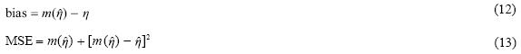
where m() and S²() are the mean and variance obtained from generated samples:

When estimating the parameters and quantiles of a distribution, one would like to have unbiased and minimum MSE estimators. The MSE involves both the variance of the estimator and the squared of the bias. If a given estimator is unbiased, the MSE is equal to the variance of the estimator.

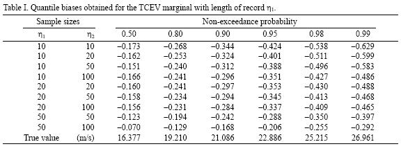
TCEV numbers with population parameters λ₁ = 450, α₁ = 2.5, λ₂ = 35 and α₂ = 2.5 were generated and grouped into samples of size n = 10, 20, 50 and 100. The number of samples for each size was equal to 10,000.

For the case of the BTCEV distribution, quantiles were obtained by combining each generated sample with another of the same "n₁" or longer length of record "n₂". So, the explored cases have lengths 10–10, 10–20, 10–50, 10–100, 20–20, 20–50, 20,100, 50–50 and 50–100. The associated TCEV numbers have population parameters λ₃ = 300, α₃ = 3, λ₄ = 60 and α₄ = 3.

A comparison was made in relation to estimating quantiles corresponding to 0.50, 0.80, 0.90, 0.95, 0.98, and 0.99 non–exceedance probabilities. In fact, when the associated length in the bivariate combination increased, the bias and mean squared error of the short series decreased throughout the range 0.5 < F < 0.99 (Tables I and II). This means that there was a gain in information when the parameters of the short series were estimated based on the short "n₁" and longer series "n₂".

 

4. Case study

The BTCEV distribution is used to model jointly the annual maximum wind speed data gathered of the hourly potential winds computed at 45 stations located in The Netherlands (Fig. 1). Data are available from the Royal Netherlands Meteorological Institute (KNMI). Some statistical characteristics of the analyzed samples are shown in Table III.

According to Simiu (2002), wind speed series used in extreme value analysis should be micrometeorologically homogeneous. That is, they should be: (a) recorded over terrain with the same roughness characteristics over the entire duration of the record being considered, (b) either recorded at or converted to the same elevation above ground, and (c) averaged over the same time interval. To assure this condition we use corrected wind speeds at 10 m height over open land with roughness length equal to 0.03 m, and averaged in an hour.

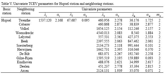
The at–site information will be related with that from EWS records of neighboring gauging stations, which can be considered to behave in similar fashion. The delineation of homogeneous regions was obtained by plotting the corresponding L–Cv coefficients and setting confidence limits (mean L–Cv plus and minus one standard deviation). Close inspection of Figure 2 indicates that there are three homogeneous regions; one of them is represented by the 14 stations listed in Table IV.

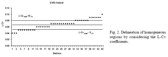
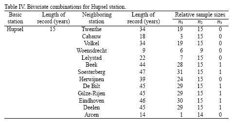
For instance, EWS data of Hupsel station can be combined with the 13 neighboring stations located at the same homogeneous region. Table IV also shows the available length of each record and the relative sample sizes of each bivariate combination.

For the bivariate combination (Hupsel–Twenth) the LL function to be maximized would be:

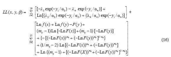
where

The required initial values of the parameters to start the optimization procedure are those obtained by the univariate approach (Table V). The final bivariate parameters and return levels (m/s) for the same cases presented in Table V are shown in Tables VI and VII.

In order to compare the goodness of fit among the univariate and bivariate estimates of return levels, the corresponding SEF values were computed. For the univariate case, the G, GEV, RW and TCEV distributions were fitted to the data. Three bivariate (B) distributions with G, GEV and RW marginals were used (BG, BGEV and BRW).

An additional comparison was made by considering three of the most popular techniques used in regional flood frequency analysis: the station–year, regional L–moments and the index flood, here called index–wind (Singh, 1987; Cunnane, 1988).

In the station–year method the standardized data recorded by all individual stations in a region can be combined so as to obtain a single regional frequency curve applicable, after appropriate rescaling, anywhere in the homogeneous region. Regional pooling was fitted by the TCEV distribution (RTCEV).

Once obtained the regional (R) weighted average values of L–moments (LM), they can be used to estimate parameters of a selection of probability distributions. In this case, the G, GEV, Gamma with two parameters (GM2) and Normal (N) distributions were fitted to the data (RGLM, RGEVLM, RGM2LM and RNLM)

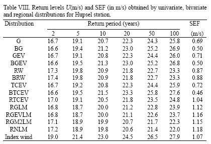
The at–site and regional at–site return levels U(m/s) of Hupsel station are shown in Table VIII. The best univariate fit was obtained with the G distribution with a SEF = 0.69 m/s. Fitting the BTCEV distribution its SEF reduced to 0.46 m/s. The return level, which is used in structural engineering, increased from 24.3 to 25.8 m/s.

A comparison between the empirical and fitted regional frequency curves for the EWS at K13 station is shown in Figure 3.

The SEF values obtained by univariate, bivariate and regional procedures along with the name of the best distribution for each analyzed station are shown in Table IX. As it can be seen, best results were obtained by fitting bivariate distributions.

 

5. Conclusions

A bivariate extreme value distribution with TCEV marginals was used to model extreme wind speeds. The maximum likelihood estimators of the parameters were obtained numerically by using the multivariable constrained Rosenbrock optimization algorithm, which worked out very well in all cases.

The quantiles of extreme value distributions can be estimated more accurately when using the BTCEV distribution. Analysis of results suggests that the effect of the additional samples in estimating the parameters and quantiles is more important when estimating the parameters of the shorter series. In fact, as the sizes of the longer series increase, the gain in information of the shorter series increases. On the contrary, this is not necessarily true when estimating the parameters of the longer series.

Data–based results indicate that there is a reduction in the standard error of fit when estimating the parameters of the marginal distribution, taking in to account the information from an additional gauging station, instead of its univariate or regional counterpart, and differences between at–site and regional at–site design events can be significant as return period increases.

None case was better fitted for the station–year, index wind or regional L–moments methods. Best fits were obtained by using bivariate distributions.

Results suggest that it is very important to consider the BTCEV distribution as an additional mathematical tool when analyzing extreme wind speeds. The final return levels were not observed like unrealistic design events even for long return periods.

 

References

Beran M. A., J. R. M. Hosking and N. W. Arnell, 1986. Comment on: Two–Component Extreme Value Distribution for flood frequency analysis, by Rossi et al. Water Resour. Res. 22, 263–266.        [ Links ]

Boni G., A. Parodi and R. Rudari, 2006. Extreme rainfall events: learning from raingauge time series. J. Hydrol. 327, 306–314.        [ Links ]

Cunnane C, 1988. Methods and merits of regional flood frequency analysis. J. Hydrol. 100, 269–290.        [ Links ]

Escalante C., 1998. Multivariate extreme value distribution with mixed Gumbel marginals, J. Am. Water Res. As. 34, 321–333.        [ Links ]

Escalante C, 2007. Application of bivariate extreme value distribution to flood frequency analysis: A case study of Northwestern México. Nat. Hazards 42, 37–46.        [ Links ]

Fiorentino M., K. Arora and V. P. Singh, 1987. The two–component extreme value distribution for flood frequency analysis: Derivation of a new estimation method. Stochastic Hydrol. Hydraul. 1, 199–208.        [ Links ]

Francés F., 1998. Using the TCEV distribution function with systematic and non–systematic data in a regional flood frequency analysis. Stochastic Hydrol. Hydraul. 12, 267–283.        [ Links ]

Furcolo P., P. Villalini and F. Rossi, 1995. Statistical analysis of the spatial variability of very extreme rainfall in the Mediterranean area. U.S.–Italy Research Workshop on the Hydrometeorology, Impacts and Management of Extreme Floods. Perugia, Italy, 13–17 Nov., 23pp.        [ Links ]

Gumbel E. J., 1960. Multivariate extremal distributions, Bull. Int. Statist. Inst. 39, 471–475.        [ Links ]

Gumbel E. J. and C. K. Mustafi, 1967. Some analytical properties of bivariate extremal distributions, Am. Stat. Assoc. J. 62, 569–589.        [ Links ]

Kite G. W., 1988. Frequency and Risk Analyses in Hydrology. Water Resources Publications, USA, 264 pp.        [ Links ]

Kuester, J. L. and J. H. Mize, 1973. Optimization Techniques with FORTRAN. McGraw–Hill, USA, 500 pp.        [ Links ]

Raynal J. A., 1985. Bivariate extreme value distributions applied to flood frequency analysis Ph. D. dissertation, Civil Engineering Department, Colorado State University, USA, 273 pp.        [ Links ]

Rossi F., M. Fiorentino and P. Versace, 1984. Two–Component Extreme Value Distribution for flood frequency analysis. Water Resour. Res. 20, 847–856.        [ Links ]

Rossi F., M. Fiorentino and P. Versace, 1986. Reply to the comment on: Two–Component Extreme Value Distribution for flood frequency analysis. Water Resour. Res. 22, 267–269.        [ Links ]

Simiu E., 2002. Meteorological extremes. In: Encyclopedia of Environmetrics. (El–Shaarawi AH, and W. W. Piegorsch Edits.). John Wiley and Sons, UK, 1255–1259.        [ Links ]

Singh V. P., 1987. Regional flood frequency analysis. D. Reidel Publishing Company, Holland, 400 pp.        [ Links ]

Van Den Brink H. W., G. P. Konnen and J. D. Opsteegh, 2004. Statistics of extreme synoptic–scale wind speeds in ensemble simulations of current and future climate. J. Climate 17, 4564–4574.        [ Links ]