


Serviços Personalizados
Journal
Artigo
 Inglês (pdf)
 Artigo em XML
 Referências do artigo
 Enviar este artigo por email
Indicadores
-
 Citado por SciELO
 -
 Acessos
Links relacionados
-
 Similares em
SciELO
Similares em
SciELO
Compartilhar

 Permalink
Atmósfera
versão impressa ISSN 0187-6236
Atmósfera vol.20 no.1 Ciudad de México Jan. 2007
Ensemble lagged forecasts of a monsoon depression over India using a mesoscale model
VINODKUMAR and A. CHANDRASEKAR
Department of Physics and Meteorology, Indian Institute of Technology, Kharagpur, India
Corresponding author: A. Chandrasekar; e mail: chand@phy.iitkgp.ernet.in
Received May 6, 2005; accepted June 16, 2006
RESUMEN
Durante el 27 de julio de 1999 se formó una depresión monzónica sobre la bahía de Bengala, India, que cruzó la costa este del país el 28 de julio del mismo año. El sistema ocasionó lluvias abundantes sobre la costa este y regiones adyacentes y es investigado en este trabajo utilizando métodos de ensamble retrasados con el Modelo de Mesoescala de Quinta Generación (MM5) de la Pennsylvania State University y el National Center for Atmospheric Research (PSU/NCAR). Se diseñan dos grupos de experimentos con cinco miembros de ensambles cada uno empezando el 25 de julio de 1999 a las 12 UTC con intervalos subsiguientes de 3 horas. En el primer experimento se utilizan los datos del reanálisis del Nacional Center for Environmental Prediction (NCEP) para el pronóstico de un dominio de malla gruesa y un anidaje subsecuente a un dominio de malla más fino (30 km). En el segundo experimento los datos del reanálisis del NCEP se utilizan directamente en el dominio de 30 km como condiciones iniciales y de frontera. Se encuentra que en los tiempos iniciales de verificación, el promedio del ensamble del campo de presión al nivel del mar correspondiente al segundo experimento tiene una estructura horizontal más grande y es más cercano al reanálisis del NCEP. Sin embargo, se encontró que en tiempos posteriores de verificación el promedio del ensamble del campo de presión al nivel del mar es mejor en el primer experimento. Todos los miembros del ensamble del primer experimento tienen valores mayores en el área promedio de precipitación acumulada de 24 horas que los del segundo experimento. Asimismo, los valores de la dispersión de todos los miembros del ensamble del primer experimento para el área promedio de precipitación acumulada de 24 horas son mayores que los del promedio de su respectivo ensamble en el segundo experimento. Los resultados de este estudio pueden ser útiles para los centros de pronóstico operativo del tiempo en la India, ya que pueden proporcionar diferentes maneras de desarrollar y probar la importancia de los ensambles.
ABSTRACT
A monsoon depression formed over the Bay of Bengal, India, during 27 July 1999 and crossed the east coast of India on 28 July 1999. The system caused copious rainfall over the east coast of India and adjacent regions and is investigated in this study using ensemble lagged methods with the Pennsylvania State University/ National Center for Atmospheric Research (PSU/NCAR) Fifth Generation Mesoscale Model (MM5). Two sets of experiments are designed with five members of ensembles in each set starting at 12 UTC 25 July 1999 and at preceding times separated by 3 hour intervals. In the first experiment, the National Center for Environmental Prediction (NCEP) reanaly sis data is utilized in the forecast of a coarse grid spacing domain and subsequent nest down to a finer (30 km) grid spacing domain. In the second experiment, the NCEP reanalysis data is directly utilized in the 30 km domain as initial/boundary conditions. The results of the ensemble average of both experiments are compared with the analysis and observations. It is found that at the initial times of verification, the ensemble average of the sea level pressure field corresponding to the second experiment has a larger horizontal structure and is more closer to NCEP reanalysis. However at later times of verification, the ensemble average of sea level pressure field corresponding to the first experiment is found to be better. The area averaged 24 hour accumulated precipitation of all the ensemble members have higher values corresponding to the first experiment as compared to the second experiment. Also, the spread of the area averaged 24 hour accumulated precipitation of all the ensemble members with respect to their respective ensemble average are higher for the first experiment as compared to the second experiment. The results of the study would be useful to operational weather forecasting centers in India as it would provide them different evaluating ways to develop and test the importance of ensembles.
Keywords: Ensemble, MM5, depression.
1. Introduction
A set of forecasts that is verified at the same time can be broadly termed as a forecast ensemble. Various sets of time lagged forecasts starting at different initial times and being verified at the same time can form an ensemble. The above implementation of ensemble methods is primarily focused on the uncertainties in the initial condition. However, in recent times the above approach has been extended to account for the uncertainties in the model itself. Hence forecasts from different models as well as different formulations of the physics (for example physical parameterization schemes) of the same model could also constitute an ensemble. Ensemble weather forecasting in operational centers have gained in importance in recent times. While the idea of ensemble forecasting has been there for a long time, the actual implementation of ensemble methods for operational weather forecasting centers has been on the increase in recent times due to increased computational resources. It is well known that the ensemble mean should give a better forecast than the control forecast provided the ensemble represents the uncertainty present in the control analysis (Epstein, 1969; Leith, 1974). One of the simplest ways to generate perturbations is to use random perturbations. It has now been realized that random perturbations is not the best way of making ensemble forecasts for random perturbations still require several hours or even days before they can organize and grow as fast as the forecast errors (Toth and Kalnay, 1993). Hoffman and Kalnay (1983) proposed the lagged average forecasting (LAF) method, which utilizes the forecasts started at earlier and at different lag times. However, the LAF ensemble method has the disadvantage that the earlier started forecasts have a much larger perturbation and hence are relatively less skillful than the latter forecasts (Toth and Kalnay, 1993). One approach to circumvent the above is to ascribe different weights for the different members in the ensemble (Hoffman and Kalnay, 1983) or by scaling back the large errors to a moderate and reasonable size (Ebisuzaki and Kalnay, 1991). Another well known method called the breeding of growing modes was proposed by Toth and Kalnay (1993), which provides for realistic perturbations that actually represent the errors present in the analysis.
Arritt et al. (2004) utilized four different methods for creating ensembles for seasonal limited area forecasts. The above study addressed the summer 1993 flood (1 June 1993 – 31 July 1993) over the north central United States. While the first three methods utilized the Pennsylvania State University/National Center for Atmospheric Research (PSU/NCAR) Fifth Generation Mesoscale Model (MM5) (using LAF, perturbed physics method and mixed physics method) for generating ensembles, the fourth method used multi–model ensembles. The model results of the above study revealed that the lagged average ensemble had very little spread, while the multi–model and the mixed physics methods had the largest spread. The reason for the small spread in the lagged average method using the MM5 model is attributed to the dominance of the lateral boundary condition on the regional model solution with very little impact of the initial condition. The above is understandable considering the seasonal nature of the integrations lasting two months. The highest equitable threat score (ETS) was related to the specific threshold for the accumulated precipitation. For low values of precipitation threshold, both lagged ensemble as well as mixed physics ensemble produced the highest ETS while for the higher precipitation threshold, both mixed physics and multi–model ensembles produced the highest ETS (Arritt et al., 2004). Pendergrass (2004) used two bias correction methods, namely lagged average and lagged linear regression for individual members of ensemble forecasts. Both methods utilize the forecast bias from previous forecasts to predict the bias of the current forecast at every station. The results of the study indicate that the lagged linear regression methods are less biased but have more variance than the forecasts corrected with the lagged average method.
Among the well known and widely used non–hydrostatic mesoscale models are the Fifth Generation Mesoscale Model (MM5) (Grell et al., 1994), the Regional Atmospheric Modeling System (RAMS) (Pielke et al., 1992) and the Advanced Regional Prediction System (ARPS) (Xue et al., 2000). Roy Bhowmik and Prasad (2001) investigated the performance of the adapted version of the Florida State University (FSU) Limited Area Model (LAM) in predicting precipitation estimates over India during South–West Monsoon (June–September) and North–East Monsoon (October and November) for three years (1997–1999). Due to the relatively coarse grid spacing of the model (1 x 1°), some underestimation of the orographic rainfall was observed. However, the above LAM was successful in reproducing the spatial patterns of monthly and seasonal rainfall. Roy Bhowmik (2003) using the FSU LAM examined the impact of model horizontal grid spacing (50 km and 16 vertical levels as well as 100 km and 12 vertical levels) for the case of three monsoon depressions and one tropical cyclone during August and September 1997. The results indicated that the observed heavy precipitation pattern over the Western Ghats could be reproduced by a model with a finer grid spacing. Potty et al. (2000) utilized a limited area mesoscale model to simulate the structure and track of four monsoon depressions over the Bay of Bengal. The results indicated that while the magnitude of the central pressure was higher than observed, the location, track, and the spatial distribution of precipitation associated with the monsoon depression could be well simulated. Potty et al. (2001) simulated the planetary boundary layer (PBL) structure over the Indian summer monsoon trough using a mesoscale model during the passage of a monsoon depression. The main observed features of the monsoon trough region were well simulated by the model. While there have been a large number of studies which have investigated the impact of additional observations on the simulation and structure of monsoon depressions, tropical cyclones, and low pressure systems which have occurred over India, there are not many studies which have utilized ensemble methods to investigate systems which have formed over India. While Section 2 provides a description of the monsoon depression, section 3 outlines a description of the model and the design of ensemble numerical experiments. Section 4 provides the results while section 5 describes the conclusions of this study.
2. Description of the monsoon depression
A low–pressure system had formed initially on 25 July 1999 over the Bay of Bengal, India. The above low pressure system had subsequently intensified to a depression on 27 July 1999. A deep cloud cluster of 200 km in horizontal extent was seen to the west of the center of the monsoon depression. Outgoing long–wave radiation (OLR) minima of 135 W nr2 were also found to the west of the depression center, indicating strong convection while high values of OLR were observed from the south and the central Bay. The system further intensified to a deep depression on 28 July 1999 before crossing land on the same day (Thapliyal et al., 2000). The deep depression weakened into a low pressure system on July 30 over Central India, northwest Madhya Pradesh, and continued to move west, northwestwards and subsequently weakened over west Rajasthan on 3 August 1999. The above depression caused copious rainfall along its track and is investigated in this study using ensemble methods.
3. Description of the model and ensemble experiments
The present study utilized the MM5 model version 3.5 (Grell et al., 1994; Dudhia, 1993, Dudhia and Bresch, 2002). The MM5 model is a limited area, nonhydrostatic, terrain following sigma coordinate model designed to simulate or predict mesoscale atmospheric circulation. The advantage of the MM5 model, other than its availability in public domain is that it offers multiple–nesting capability, four–dimensional data assimilation (Newtonian nudging), a large number of physics options along with the availability of both one–way as well as two–way nesting options. Twenty three vertical layers (centered at σ = 0.995, 0.985, 0.97, 0.945, 0.91, 0.87, 0.825, 0.775, 0.725, 0.675, 0.625, 0.575, 0.525, 0.475, 0.425, 0.375, 0.325, 0.275, 0.225, 0.175, 0.125, 0.075, 0.025) and a system of two nested domains of horizontal grid spacing 90 km (85 X 75 grid cells in east–west and north–south directions) and 30 km (129 x 119 grid cells in the east–west and north–south directions) were utilized. The study used the Medium Range Forecast (MRF) scheme for PBL, the Grell (Grell, 1993) scheme for cumulus parameterization, a simple ice scheme for explicit moisture, a simple radiation scheme and a multi–level soil model. Mandal et al. (2004) utilized the MM5 model to study the impact of the various physical parameterization schemes on the prediction of tropical cyclones over Bay of Bengal. They utilized two planetary boundary layer (PBL) and four convection schemes to simulate two tropical cyclones (7–9 and 22–25 November 1995) which formed over the Bay of Bengal, and found that the Hong–Pan PBL scheme (known as MRF PBL) in combination with Grell (or Betts–Miller) cumulus scheme was found to perform better than other combinations. In our MM5 simulations, we have used the MRF PBL scheme in combination with Grell cumulus scheme for simulating tropical systems such as monsoon depressions as suggested by the results of Mandal et al. (2004). Also National Center for Environmental Prediction (NCEP) reanalysis data (Kalnay et al., 1996) available at a horizontal grid spacing of 2.5 x 2.5° (144 x 73 grid cells from 90N 90S and 0E 357.5E) and a time spacing of 6 hours were used to provide for initial and lateral boundary conditions. The pressure level data available at seventeen pressure levels (hPa): 1000, 925, 850, 700, 600, 500, 400, 300, 250, 200, 150, 100, 70, 50, 30, 20, 10 for the following five variables namely: air temperature, zonal wind component, meridional wind component, water vapor specific humidity and geopotential height were utilized. In addition, surface flux data such as sea level pressure, skin temperature, air temperature and water vapor specific humidity at 2 m, zonal and meridional wind components at 10 m, and soil temperature and soil moisture (0 – 10 cm and 10–200 cm) from NCEP reanalysis were utilized. A one–way nesting option was employed. In this study, five sets of time–lagged forecasts starting at different initial times and being verified at the same time were generated. The five sets of ensembles which form part of the first experiment were started at five different starting times 25 July 1999, 00, 03, 06, 09 and 12 UTC, and were integrated till 29 July 1999, 00 UTC. The analysis at 03 and 09 UTC was obtained by time averaging of the adjacent analysis. Here, the NCEP reanalysis was utilized in the forecast of the 90 km domain and subsequent nest down to the 30 km domain. The analysis at 03 and 09 UTC was obtained by time averaging of the adjacent analysis. Another set of five ensembles which form part of the second experiment were generated by directly utilizing NCEP reanalysis to the 30 km domain as initial/boundary conditions at the same five initial times as mentioned above. The integrations of all the five ensembles were performed till 29 July 1999, 00 UTC. While at near the beginning of the verification time, all the five ensembles of the second experiment have analysis errors, all the five ensembles of the first experiment have forecast errors (the latter due to integration of the coarse 90 km domain and whose output was used to create initial and lateral boundary conditions for the 30 km domain) in addition to the analysis errors. No four–dimensional data assimilation (FDDA) was utilized in these numerical experiments.
The objective of this study is to examine the differences if any of the nature of the ensemble mean obtained through the first and second experiments, as well as the nature of the spread of each ensemble member about the ensemble mean for both the experiments. The results of each of the five ensemble members of each experiment were verified at the same time (26 July 1999, 00 UTC and thereafter till 29 July 1999, 00 UTC). However for the area averaged 24 hour accumulated precipitation values, the verification started from 26 July 1999 12 UTC and thereafter till 29 July 1999, 00 UTC.
4. Results and discussions
The primary objective of this study is to investigate the use of ensemble methods i.e. importance of initial conditions (forecasts being started at different times and being verified at the same time) in the prediction of tropical systems such as monsoon depressions. In addition, this study seeks to pose if it is desirable to use the NCEP reanalysis directly to the 30 km domain as initial/boundary conditions or is it better to use the reanalysis data for the forecast of the coarse domain (90 km) and subsequent nest down to a finer grid spacing (30 km) domain. Which of the above two scenarios would provide for a better forecast. Figure 1 provides the model domain utilized in this study. Figures 2–4 (Figures 2, 3, 4) depict the sea level pressure patterns for 26 July 1999, 00 (Figs. 2a, 2c and 2e) and 12 UTC (Figs. 2b, 2d and 2f), for 27 July 1999, 00 (Figs. 3a, 3c and 3e) and 12 UTC (Figs. 3b, 3d and 3f) and for 28 July 1999, 00 (Figs. 4a, 4c and 4e) and 12 UTC (Figs. 4b, 4d and 4f). All the figures and the model results in this study pertain to the 30 km domain. Since the NCEP reanalysis data has coarse grid spacing of 2.5 X 2.5° it is proposed to start the verifying time at 26 July 1999, 00 UTC (i.e. after allowing for at least 12 hours of integration). The top panels provide the sea level pressure pattern from NCEP reanalysis while the middle and lower panels depict the ensemble average of the mean sea level pressure obtained from the MM5 simulations corresponding to the first and the second experiments. The ensemble mean is obtained by averaging all the ensemble members at the same verifying time. Except for the sea level pressure field obtained from the MM5 model at 26 July 1999, 00 UTC, the sea level pressure fields obtained at other times from the same model provide for a weaker system as compared to the analysis. The above result can be attributed to the absence of FDDA of observation with finer grid spacing. The reason for the above behavior is that model simulations with just the 2.5 X 2.5° NCEP reanalysis data as initial conditions without any assimilation of high resolution observations may not yield the desired simulation performance. Figure 2 reveals that the horizontal structure of the depression from the second experiment (NCEP reanalysis is directly utilized in the 30 km domain as initial/boundary conditions) has large spatial extent and is closer to the NCEP reanalysis than the results of the first experiment (reanalysis used in forecast of 90 km domain and subsequent nest down to 30 km domain). The above behavior can be understood considering the fact that at the start of the verifying time (26 July 1999, 00 and 12 UTC), the ensemble members of the second experiment contain only the analysis errors while the ensemble members of the first experiment contain forecast errors in addition to the analysis errors. Although a similar behavior is seen for the times 27 and 28 July 1999, 12 UTC, an opposite behavior is seen at other days (27 and 28 July 1999, 00 UTC). While there are, undoubtedly, errors associated with the forecast of the coarse grid spacing domain in the ensemble members of the first experiment, it has to be remembered that both the 90 and 30 km domains are integrated using the same model dynamics and physics. Hence there is a possibility of reduced spin–up or shock effect at the forecast start for the MM5 simulations corresponding to the first experiment due to better balance of the initial model condition as compared to the simulation of the second experiment. Also, the availability of the lateral boundary conditions is more frequent (equal to the output frequency of the coarse domain model which is 3 hours) for the first experiment as compared to the second experiment (frequency of NCEP reanalysis which is 6 hours). The contrasting behavior (seen at 00 and 12 UTC) of the results of the two experiments as far as the horizontal structure of the sea level pressure field for 27 and 28 July 1999 appears to be associated with diurnal variation.


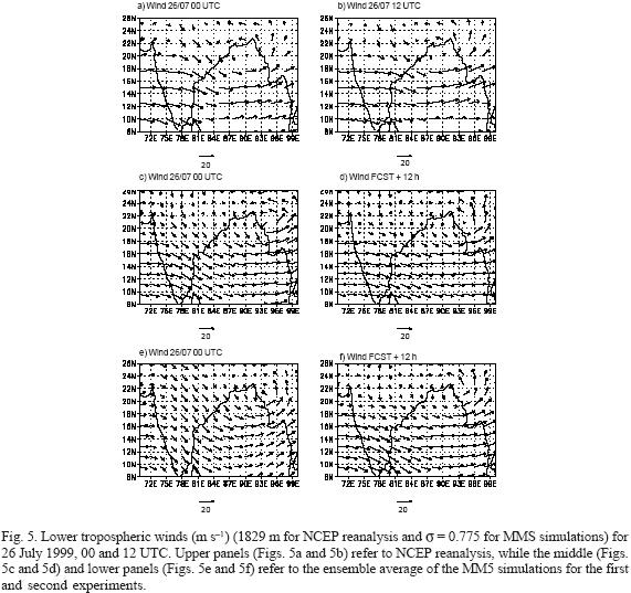
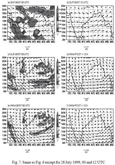
Figures (5–7) (Figures 5, 6, 7) depict the lower tropospheric winds (26–28 July 1999, 00 and 12 UTC) as well as the 24 hour accumulated precipitation (the latter restricted to 27 and 28 July 1999, 00 UTC) from the NCEP reanalysis (a and b, upper panels) and from the ensemble average obtained from MM5 simulations corresponding to the first (c and d, middle panels) and second (e and f, lower panels) experiments. The lower tropospheric winds from the NCEP reanalysis refer to a height of 1829 m, and the same from the MM5 simulations correspond to the nearest σ level (σ = 0.775) having a height of 1882 m. While the cyclonic circulation at 26 July 1999, 00 and 12 UTC in the ensemble average of both experiments (Figs. 5c, 5d, 5e, and 5f) is not different from one another, the same for latter time (27 and 28 July, 00 and 12 UTC) reveals that the ensemble average of the first experiment (Figs. 6c, 6d, 7c and 7d) provide for a stronger cyclonic circulation especially to the north of the depression center as compared to the ensemble average corresponding to the second experiment. Figure 8 depicts the sea level pressure field (Figs. 8a, 8c and 8e), the lower tropospheric wind field as well as the 24 hour accumulated precipitation (Figs. 8b, 8d and 8f) for 29 July 1999, 00 UTC. Again, the ensemble average of the first experiment (Fig. 8c) provides a larger structure of the sea level pressure field as compared to the ensemble average of the second experiment (Fig. 8e) . Also, the ensemble average of the lower tropospheric wind corresponding to the first experiment (Fig. 8d) shows a stronger cyclonic circulation especially to the north of the depression center as compared to the ensemble average of the second experiment (Fig. 8f). The above behavior is similar to the behavior seen for 27 and 28 July 1999, 00 UTC. Figure 9 (a–f) depicts the Tropical Rainfall Measurement Mission (TRMM) 24 hour accumulated rainfall (Figs. 9a, 9c and 9e) as well as QuikSCAT winds over the sea (Figs. 9b, 9d and 9f) for 27 July 1999, 00 UTC, 28 July 1999, 00 UTC, and 29 July 1999, 00 UTC. It is evident that the precipitation values obtained from the NCEP reanalysis for 27–29 July 1999, 00 UTC (Figs. 6a, 7a and 8b) are much lower compared to the rainfall amounts from TRMM (Figs. 9a, 9c and 9e). While the maximum rainfall from TRMM is seen over the east coast of India as well as adjacent Bay of Bengal regions (Fig. 9a) on 27 July 1999, 00 UTC, the rainfall pattern seems to be at a more inland location for the next two days (Figs. 9c and 9e), consistent with the fact that the depression has indeed crossed land on 28 July 1999. The ensemble average of the 24 hour accumulated precipitation for both experiments do not reveal marked inland penetration of the rainfall pattern on 28 and 29 July 1999, 00 UTC as revealed by the TRMM data. The 24 hour accumulated precipitation as manifested in the ensemble average of the second experiment (Fig. 6e) exhibits an improved large scale structure of the spatial precipitation pattern on 27 July 1999, 00 UTC. However, for the other days (28 and 29 July 1999, 00 UTC), the ensemble average corresponding to the first experiment (Fig. 7c and 8d) reveals more amount of rainfall over the eastern coastal areas with relatively more inland penetration of rainfall compared to the second experiment (Figs. 7e and 8f). However, the rainfall amounts of both experiments as deduced from the model seem to be underestimated as compared to the TRMM data.


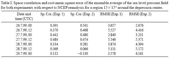
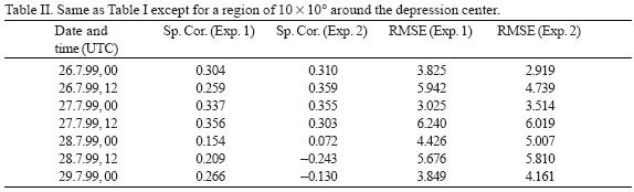
In order to obtain a quantitative measure of the difference of the ensemble average obtained from the two experiments, the following strategy was conceived. First a box of 15 x 15° domain was identified over the center of the depression (i.e. location of the minimum sea level pressure as obtained from the NCEP reanalysis). The space correlation as well as the root mean square errors (RMSE) of the ensemble average of sea level pressure field for both experiments with respect to the NCEP reanalysis data was obtained at different times and is shown in Table I. It is clear from Table I that the space correlation of the sea level pressure field corresponding to the ensemble average of the second experiment is higher compared to the first experiment till 27 July 1999, 00 UTC. Also, the RMSE of the ensemble average of the second experiment is lower for the first day as compared with the first experiment. This result is consistent with our earlier deduction that at the initial verifying time the second experiment has only analysis errors, while the first experiment has forecast errors in addition to the analysis errors. The situation, however, changes after 27 July 1999, 00 UTC with the space correlation of the first experiment having higher value and the corresponding RMSE of the first experiment being lower as compared to the second experiment. The above behavior has been observed and mentioned earlier. Table I also indicates that the RMSE of the sea level pressure field for both experiments manifests a diurnal variation. Table II is similar to Table I except that the box under consideration is of 10 x 10° extent. The results of Table II are similar to Table I except that the magnitudes of the space correlation are lower and the RMSE slightly higher as compared to Table I.
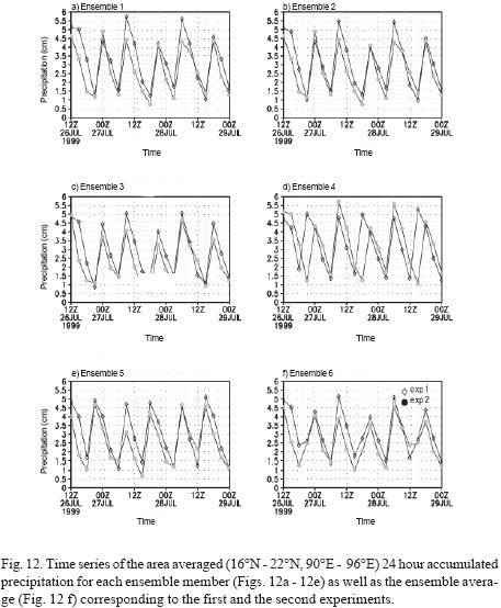
It would be of interest to analyze the area averaged 24 hour accumulated precipitation of each of the five ensemble members (for both experiments) as well as to examine the spread of each of the ensembles with respect to the ensemble average for both experiments. It is proposed to consider the area average of the following box between the longitudes 90 and 96° E and between the latitudes 16 and 22° N. The above limits are chosen for the box keeping in mind the location of the monsoon depression in the North Bay of Bengal during the period 26–29 July 1999. The domain considered is smaller as the precipitation field associated with the depression (unlike the domain considered in sea level pressure field) does not extend to a large region. Figure 10 shows the time series of the area averaged 24 hour accumulated precipitation for each of the five ensembles as well as the ensemble average of the first experiment from 26 July 1999, 12 UTC to 29 July 1999, 00 UTC. All the ensemble members appear to have two minima and two maxima over the duration of each day. While the first three ensemble members show somewhat similar behavior, the fourth and the fifth ensemble exhibit different behavior. The standard deviation of the first five ensembles (spread of each of the ensemble members with respect to the ensemble average) of the area averaged 24 hour precipitation for the first experiment is calculated and has the following values: 0.734, 0.639, 0.596, 0.945 and 0.950 cm. Figure 11 is similar to Figure 10 except that the former corresponds to the results of the second experiment. Again, all the ensemble members show two minima and two maxima over the duration of a day. The results of the second experiment are similar to the first one, except that at most times the area averaged 24 hour accumulated precipitation has lower values in the second experiment as compared with the first experiment. The standard deviation of the first five ensembles (spread of each of the ensemble members with respect to the ensemble average) of the area averaged 24 hour precipitation for the second experiment is calculated and has the following values: 0.646, 0.553, 0.549, 0.723 and 0.907 cm. The above values indicate that the spread of the area averaged 24 hour precipitation of all the ensemble members about their respective ensemble average is more in the first experiment as compared to the second experiment. In order to bring out any differences at all between the same ensemble members corresponding to both experiments, it was decided to plot the area averaged 24 hour accumulated precipitation (Fig. 12) for each of the five ensemble members as well as the ensemble average corresponding to both experiments. The results indicate that the maximum value of the area averaged 24 hour accumulated precipitation corresponding to the first experiment has higher values as compared to the second experiment. The above holds true at most times and for all the ensemble members as well as the ensemble average.


5. Conclusions
This study investigated the use of ensemble methods (forecasts being started at different times and being verified at the same time) on the prediction of a monsoon depression. In addition, this study examined differences, if any, present between two sets of experiments. The first experiment used NCEP reanalysis data for the forecast of a coarse domain (grid spacing 90 km) and then utilized the 90 km domain output through nest down to a finer domain with 30 km grid spacing. The second experiment, on the other hand, directly used the NCEP reanalysis data for initial and lateral boundary conditions in the domain with 30 km grid spacing. The re sults of the study indicate that at the initial times of verification, the ensemble average of the sea level pressure field corresponding to the second experiment has a larger horizontal structure and is more closer to NCEP reanalysis. This result is consistent with the fact that at the initial verifying time the second experiment has only analysis errors while the first experiment has forecast errors (due to the integration of the coarse domain) in addition to the analysis errors. However at later times of verification, the ensemble average of sea level pressure field corresponding to the first experiment is found to be better. It is true that there are errors associated with the forecast of the domain with the coarse grid spacing in the ensemble members of the first experiment. However, it is pertinent to note that both the 90 km and 30 km domains in the first experiment are integrated using the same model dynamics and physics. Hence there is a possibility of reduced spin–up or shock effect at the forecast start for the MM5 simulations corresponding to the first experiment due to better balance of the initial model condition as compared to the simulation of the second experiment. Also the availability of the lateral boundary conditions is more frequent (equal to the output frequency of the coarse domain model which is 3 hours) for the first experiment as compared to the second experiment (frequency of NCEP reanalysis which is 6 hours). The above can impact on the simulation results at later verifying times. The area averaged 24 hour accumulated precipitation indicates higher values for all ensemble members corresponding to the first experiment as compared to the second experiment. Also the spread of the 24 hour accumulated precipitation of all the ensemble members about their respective ensemble average is more in the first experiment as compared to the second experiment.
Acknowledgement
The authors acknowledge NCAR for making the MM5 model available to public domain. The authors thank NCEP for providing the reanalysis data used in this study. The authors thank NASA for TRMM and QuikSCAT data. The authors have utilized MM5toGrADS script and plotted all the figures using GrADS. Vinodkumar acknowledges the Council of Scientific and Industrial Research, India, for providing financial assistance to undertake this study.
References
Arritt R. W., C. J. Anderson, E. S. Takle, Z. Pan, W. J. Gutowski Jr., F. O. Otieno, R. da Silva, D. Caya, J. H. Christensen, D. Luth, M. A. Gaertner, C. Gallordo, S. Y. Hong, C. Jones, H. M. H. Juang, J. J. Katzfey, W. M. Lapenta, R. Laprise, J. W. Larson, G. E. Liston, J. L. McGregor, R. A. Pielke Sr., J. O. Roads and J. A. Taylor, 2004. Ensemble methods for seasonal limited area forecasts, AMS 20th. Conference on Weather Analysis and Forecasting, 16th. Conference on NWP 12–16 January 2004, Seattle, Washington. [ Links ]
Dudhia J., 1993. A nonhydrostatic version of the Penn State/NCAR mesoscale model: Validation tests and simulation of an Atlantic cyclone and cold front. Mon. Wea. Rev. 121, 1493–1513. [ Links ]
Dudhia J. and J. F. Bresch, 2002. A global version of the PSU–NCAR mesoscale model. Mon. Wea. Rev. 130, 2989–3007. [ Links ]
Ebisuzaki W. and E. Kalnay, 1991. Ensemble experiments with a new lagged analysis forecasting scheme. Research Activities in Atmosphere and Oceans, Modeling Report No. 15, WMO. [ Links ]
Epstein, E.S., 1969. Stochastic dynamical prediction. Tellus 21, 739–759. [ Links ]
Grell G. A, 1993. Prognostic evaluation of assumptions used by cumulus parameterizations. Mon. Wea. Rev. 121, 764–787. [ Links ]
Grell G. A., J. Dudhia and D. R. Stauffer, 1994. A description of the fifth–generation Penn State/ NCAR mesoscale model (MM5). NCAR Technical Note TN–398+STR, National Center for Atmospheric Research, Boulder, CO, USA. [ Links ]
Hoffman R. N. and E. Kalnay, 1983. Lagged average forecasting; an alternative to Monte Carlo forecasting. Tellus 35A, 100–118. [ Links ]
Kalnay E., M. Kanamitsu, R. Kistler, W. Collins, D. Deaven, L. Gandin, M. Iredell, S. Saha, G. White, J. Woollen, Y, Zhu, A. Leetmaa and R. Reynolds, 1996. The NCEP/NCAR 40–Year Reanalysis Project. Bull.Amer. Met. Soc. 77, 437–471. [ Links ]
Leith C. E., 1974. Theoretical skill of Monte Carlo forecasts. Mon. Wea. Rev. 102, 409–418. [ Links ]
Mandal M., U. C. Mohanty and S. Raman, 2004. A study on the impact of parameterization of physical processes on prediction of tropical cyclones over the Bay of Bengal with NCAR/PSU mesoscale model. Natural Hazards 31, 391–414. [ Links ]
Pendergrass A. G. and K. L. Elmore, 2004. Ensemble forecast bias correction, http://www.caps.ou.edu/reu/reu04/AngiePendergrass.FinalPaper.pdf (consulted 09/10/04). [ Links ]
Pielke R. A., W. R. Cotton, R. L. Walko, C. J. Tremback, W. A. Lyons, L. D. Grasso, M. E. Nicholls, M. D. Moron, D. A. Wesley, T. J. Lee and J. H. Copeland, 1992. A comprehensive meteorological modeling system –RAMS. Meteorol. Atmos. Phys. 49, 69–91. [ Links ]
Potty K. V. J., U. C. Mohanty and S. Raman, 2000. Numerical simulation of monsoon depressions over India with a high resolution nested regional model. Meteorol. Appl. 7, 45–60. [ Links ]
Potty K. V. J., U. C. Mohanty and S. Raman, 2001. Simulation of boundary layer structure over the Indian summer monsoon trough during the passage of a depression. J. Appl. Met. 40, 1241–1254. [ Links ]
Roy Bhowmik S. K. and K. Prasad, 2001. Some characteristics of limited area model precipitation forecast of Indian monsoon and evaluation of associated flow features. Meteorol. Atmos. Phys. 76, 223–236. [ Links ]
Roy Bhowmik S. K., 2003. Prediction of monsoon rainfall with a nested grid mesoscale limited area model. Proc. Indian Acad. Sci. (Earth Planet. Sci.) 112, 499–519. [ Links ]
Toth Z. and E. Kalnay, 1993. Ensemble forecasting at NMC: The generation of perturbations. Bull. Amer. Meteor. Soc. 74, 2317–2330. [ Links ]
Thapliyal V., D. S. Desai and V. Krishnan, 2000. Cyclones and depressions over north Indian Ocean during 1999. Mausam 51, 215–224. [ Links ]
Xue M., K. K. Droemeier and V. Wong, 2000. The Advanced Regional Prediction System (ARPS) – A multi–scale nonhydrostatic atmospheric simulation and prediction model Part I: Model dynamics and verification. Meteorol. Atmos. Phys. 75, 161–193. [ Links ]

