A note on inertial motion

A. Wiin-Nielsen
The Collstrop Foundation, H. C. Andersens Blvd. 37, 5th, DK 1553, Copenhagen V, Denmark

Received January 13, 2003; accepted January 1, 2004

 

RESUMEN

Este trabajo contiene una investigación sobre el movimiento inercial en la esfera incluyendo todos los términos de las fuerzas de Coriolis. El vector de velocidad tiene una componente zonal, una meridional y una de altura. La dependencia del tiempo de estas componentes se calcula solucionando tres ecuaciones de velocidad que contienen únicamente los términos de Coriolis. Entonces, a partir del vector de velocidad se calcula el vector de posición de tres dimensiones. Los resultados dependen de la latitud de la posición inicial. Para la mayoría de las posiciones iniciales es una buena aproximación considerar a la latitud como constante, ya que los resultados muestran que las variaciones sur-norte son bastante pequeñas para valores razonables del vector de velocidad que puede ser considerado como el viento a-geostrófico y por lo tanto muy pequeño. Estas observaciones se consideran con detalle en el trabajo. Para cada caso se dan el vector de velocidad inicial (u_o, v_o, w_o) y la posición inicial (x_o, y_o, z_o). Sin embargo, debido a la naturaleza de los términos de Coriolis se observa que no se puede dar un valor arbitrario a la componente vertical (w_o), ya que está relacionado con las otras dos componentes. El primer paso es determinar las variaciones en el tiempo de las tres componentes de velocidad, de donde posteriormente se determina la trayectoria del movimiento en tres dimensiones.

 

ABSTRACT

This note contains an investigation of the inertial motion on the sphere including all the terms of the Coriolis forces. The velocity vector has a zonal, a meridional and a height components. The time dependence of these components are calculated by a solution of the three velocity equations containing only the Coriolis' terms, and the three-dimensional position vector is then calculated from the velocity vector. The results depend on the latitude of the starting position. For most starting positions it is a good approximation to consider the latitude as a constant, because the results show that the south-north variations are quite small for reasonable values of the initial velocity vector which may be considered as the a-geostrophic wind and thus quite small. These remarks will be considered in detail in the paper. For each case the initial velocity vector (uo, vo, wo) and the starting position (xo, yo, zo) are given. However, due to the nature of the Coriolis terms it is seen that the vertical component (wo) cannot be given an arbitrary value since it is related to the other two components. The first step is to determine the time variations of the three velocity components, whereafter the trajectory of the three dimensional motion is determined.

 

1.  Introduction

The inertial motion to be described in this paper is not included in the equations as they are normally used. The reason is that the third equation of motion in the normal models is replaced by the hydrostatic equation based on an order of magnitude estimate of the terms which appear in the third equation of motion. As a consequence of this approximation it is necessary to disregard a part of the Coriolis terms in the first equation of motion to secure that the model is energetically correct. While these approximations are well justified in most situations, it is still of interest to determine the general nature of the full Coriolis terms in all three equations of motion. In the present paper the solutions with respect to time of the three-dimensional velocity vector created by the Coriolis terms will be determined. In addition, when the velocity vector is determined, it is in general possible to calculate the three-dimensional trajectory. Special solutions are necessary if the starting position is at the Equator or at the poles.

 

2. The Coriolis equations

When we include only the Coriolis terms in the three equations of motion, they take the form given in equations (1).

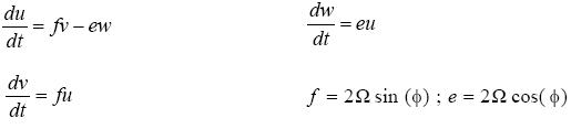..........(1)

It can be seen directly from the equations (1) that the Coriolis terms give no contribution to a change in the kinetic energy. This result is obtained when the first equation is multiplied by u, the second by v and the third by w, whereafter the three equations are added. It is then found that d[1/2(u²+v²+w²)]dt is zero. If any changes in the equations are wanted, they should be done in such a way that the kinetic energy is constant. One may for example include only the first two equations of motion. If so, any term containing e has to be excluded. We have then the classical problem appearing in most textbooks as seen in (2).

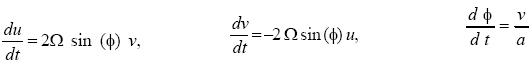.......(2)

The easy solution is obtained by using φ=φ₀; . It is this solution which is produced in the textbooks. It is, however, also possible to integrate the three equations in (2) by numerical methods. Figure 1 shows the two velocity components, and it is seen that the trajectory is a circle for all practical purposes. Figure 2 gives the latitude as a function of u. It is seen that the variation of the latitude is about 2 degrees, and it is thus a good approximation to use a constant latitude to solve the problem.

We shall then turn to the three-dimensional case. Also this case can be carried out making some simplifying assumptions, but we shall consider the general case on the sphere. If we want to include the trajectories in three dimensions we find a total of six dependent variables, i. e. three for the velocity components (u, v, w) and three to compute the trajectories. We shall in the present case use longitude (λ), latitude (φ) and the height (z) over the surface of the Earth as seen in (3).

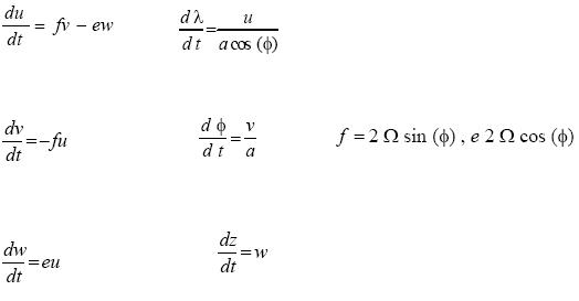........(3)

It should also be pointed out that it follows from the basic equations of the problem that the vertical velocity cannot be selected in an arbitrary way. It is seen from the second and the third equations that ev + fw is constant. We obtain therefore the relation shown in (4).

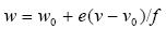.................................................................................(4)

The expression in (4) shall replace the third equation of motion. The equations in (4) may be integrated numerically to obtain both the velocity components and the three-dimensional trajectories where the particle are determined by longitude, latitude and height. The integration scheme has been the Runge-Kutta system with a time step of 5 minutes. The initial conditions require values of the three velocity components and the position. In the selection of the initial velocity components it should be recalled that the observed atmosphere is quasi-geostrophic, meaning that a major part of the velocity is in equilibrium with the pressure field. The values for the present problem are therefore to be consider as the a-geostrophic wind components. The selected values should thus be quite small to give a realistic integration. It was decided to select small values of u and v, and w =0.

Figures 3a and 3b shows the case where the initial latitude is 45 degrees north. The figure shows the latitude as a function of longitude with the initial values x = 0. 0 and y = 45 degrees. The variations are small for both variables with a change in the south-north direction of only about 0.06 degrees, while the change in the longitudinal direction is about 0.06 degrees. In this, as well as later figures the x, y and z coordinates are expressed in kilometers. We notice thus variations of 8 km in the x-directions and 6 km in the z-direction. The large vertical variation is due to the fact that the v and w are related to each other.

The integrations were repeated for an initial latitude of 80 degrees as shown in Figures 4a and 4b. It is seen that the horizontal and vertical variations are much smaller than at middle latitudes due to the large value of sine and the small values of cosine of the latitude.

As the final example we shall illustrate the behavior at the latitude of 10 degrees. We still use the same values of u_o and v_o. Figure 5a shows the values of u as a function of time for 24 hours. We notice a period of about 12 hours. Figure 5b shows the time variation of the meridional velocity component (v) which varies between 0.16 m per s and 0.33 m per s. The vertical velocity, shown in Figure 5c, is zero at t=0 and shows also a periodic variation of about 12 hours. Figure 5d indicates that the trajectory components in the horizontal plain of longitude and latitude oscillate with small amounts. The variation in the vertical direction is large as can be seen from Figure 5e, where the maximum in the height is more than 10 km.

 

3. Final remarks

The Coriolis terms which normally are excluded from the equations of motion have been investigated in isolation. The trajectories have been computed at various latitudes. It is seen that these terms may be of importance in connection with other terms such a gravity. An area of interest is the calculation of trajectories where the rotation of the Earth is of importance. Examples are the motion of satellites or the path of particles in the atmosphere.