Are transitions abrupt in Stommel's thermohaline box model?

 

S. N. Bulgakov

Instituto de Astronomía y Meteorología, Universidad de Guadalajara, Av. Vallaría 2602, Sector Juárez, C.P. 44130, Guadalajara, Jalisco, MÉXICO.

 

Yu. N. Skiba

 Centro de Ciencias de la Atmósfera, UNAM, Circuito Exterior, Ciudad Universitaria, C.P. 04510, México D. F., MÉXICO

Corresponding author: S. N. Bulgakov; e-mail: sbulgako@udgserv.cencar.udg.mx.

 

Received May 24, 2002; accepted September 11, 2003

 

RESUMEN

Se realizó una serie de experimentos en el laboratorio con temperatura y salinidad forzadas usando un aparato (un canal entre dos cajas simulando un polo y el ecuador) diseñado para reproducir el modelo conceptual de la circulación termohalina de Stommel (1961). Se discuten los patrones de la circulación dependiendo de los parámetros de modelación (flotabilidad y razón del aspecto) y las condiciones específicas en la frontera. Hay tres estados estacionarios establecidos en el espacio de control de los parámetros de la modelación: el modo térmico en dos capas (T2), el modo salino en dos capas (S2) y el modo híbrido en tres capas (H3). La circulación termohalina exhibe tanto transiciones suaves como abruptas, dependiendo de la tasa de mezcla. Los experimentos de convección libre y difusión doble con mezclado limitado mostraron transiciones suaves entre los modos de circulación. Las transiciones abruptas se encontraron sólo en experimentos de mezcla completa cuando el agua en las dos cajas fue revuelta con mezcladores.

 

ABSTRACT

A series of laboratory experiments with forced temperature and salinity were conducted using an apparatus (channel between pole and equator boxes) designed to duplicate the conceptual Stommel's model of thermohaline circulation. The flow patterns are discussed depending on modelling parameters (aspect ratio and buoyancy), and specified boundary conditions. Three steady states are found in the control space of the modelling parameters: two-layer thermal mode (T2), two-layer saline mode (S2), and three-layer hybrid state (H3). The thermohaline circulation exhibits both, smooth and abrupt transitions, depending on the rate of mixing. Free convection and double diffusion experiments with limited mixing show smooth transitions. Abrupt transitions were only found in the complete mixing experiments when two boxes were stirred by mixers.

Keywords: Thermohaline circulation, equilibria, laboratory modelling.

 

1. Introduction

Sea-water density is modified by two distinct processes: heating-cooling, which changes temperature, and freshing-salting, which changes salinity. As these processes occur at the surface, bottom, and lateral boundaries of the seawater basins, the prediction of what types of thermohaline circulation (THC) could be realized is generally not a trivial question.

In many important oceanic regions, these two density-modifying processes work contrary to one another. For example, the world ocean is a physical system with external forcing occurring predominantly at the surface. An intensive evaporation and heating in the tropics lead both to warm (low density) and salt (high density) water formation. In contrast, at high latitudes, the formation of cool (high density) and fresh (low density) polar waters is typical. There are a lot of other examples in natural sea-water basins (including estuaries) where opposing external temperature/salinity forces occur.

The interplay of these two driving agencies is not completely understood. Because of a strong nonlinearity in the advection of temperature and salinity, thermal and salinity driven circulations are not additive. These stratified flows driven by both causes will exhibit a rich variety of dynamic behaviour, including single steady states and multiple equilibria, instabilities and chaos.

One of the most interesting phenomena of THC is probably caused by the opposing temperature and salinity forcing of an equal amplitude, when the buoyancy ratio: R = β ΔS/ α ΔT is close to unity. There is a phenomenon known as multiple states in various physical problems.

Stommel (1961) was the first to note that there may exist multiple equilibria of the THC, when the system can produce two different modes of circulation and transitions for the same boundary conditions. In Stommel's model, representing pole-equator THC, two boxes ofvolume (V ) containing well-mixed water of temperature (T) and salinity (S) were connected side-by-side by two horizontal tubes at the top and at the bottom (see Fig. 5 in Stommel, 1961)). The external reservoirs affected these two boxes through the porous walls. One box was exposed to a positive temperature (T^*) and salinity (S^*) while the other one was exposed to exactly the same negative values. Diffusion through the walls produced temperature and salinity changes in the boxes according to linear relaxation laws:

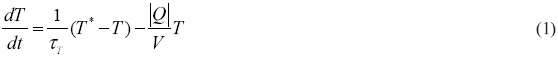
where Q is volume flux between boxes; τ_T and τ_s are the temperature and salinity relaxation time-scales, respectively. Density was governed by the linearized equation of state:

where ρ₀ is reference density, α and β are the temperature and salinity expansion coefficients, respectively.

The fluid exchange rate between the two boxes was accepted to be proportional to the density difference between boxes:

Because the heat transfer mechanism has a more rapid effect on the density, property exchange was assumed by Stommel (1961) to have a salinity time-scale much longer than the heat time-scale

Stommel solved these equations graphically. Their solutions were found as the intersections of the (1) (2) and (3) curves (see Fig. 6 in Stommel, 1961). It was noted that the three possible states of motion for the same values of reservoir temperature and salinity could arise within a certain range of forcing parameters. One state is characterized by salinity dominating the density difference between the basins which propels the water there (S-mode). The second one, is predominantly temperature driven (T-mode). Both of these states were characterized by opposite cells of the vertical circulation and were linearly stable, therefore, small perturbations of the motion decayed over time. The third state revealed an unstable mode, a so-called Stommel transition, when the system would drift to one of the other grand modes with an abrupt change in flow direction and speed. Thus, Stommel's mechanism of multiple equilibria is caused by opposing temperature and salinity forcing, at greatly different relaxation time-scales.

A necessary condition for multiple equilibria was defined by Stommel (1961) as

where R is buoyancy ratio. A sufficient condition was determined, in this case, as a small value of the parameter

Multiple equilibria have been found in a hierarchy of ocean models, ranging from the box models (Stommel, 1961; Rooth, 1982) to the 2-D theoretical (Marotzke et al, 1988), global oceanic general circulation (Bryan, 1986) and coupled ocean-atmosphere (Manabe and Stouffer, 1988) models. Theoretical models of various complexities (Welander, 1982; Winton and Sarachik, 1993; Dijkstra and Molemaker, 1997) have shown that thermohaline systems can exhibit oscillatory solutions as well.

In contrast, Straub (1996) noted an inconsistency between the Stommel's box model (which relates the strength of the exchange between two boxes to the density differences between them) and the Stommel-Arons (1960) model of the buoyancy driven circulation (which shows that the density difference is not indicative of the rate of the water exchange for the oceanic problem). Ruddick and Zhang (1996) assumed as well that Stommel's study was limited to the linear flow law (transport proportional to density difference). They slightly extended Stommel's two-box model showing that this model could not exhibit self-driven oscillations under a steady forcing. These different points of view clearly illustrate the complexity of the problem.

The analytical and numerical studies of this problem were reviewed and summarized by Marotzke (1993) and Whitehead (1995). Central to these results of the hierarchy of the theoretical models is the issue of mixed surface boundary conditions instead of the different relaxation time-scales. Theoretical studies have shown that, when prescribing both temperature and salinity, THC has a unique solution. When, for example, a prescribed salinity is replaced by a salt-flux condition, the solution can be multiple (Bryan, 1969; Marotzke et al, 1988). In such a case, the meridional THC of a pole-to-pole ocean can have several different stable states: (1) the circulation is dominated by the thermal surface forcing, providing a cell with water sinking at the poles and rising at the equator; (2) the THC is predominantly driven by the surface salinity flux, creating a cell with water sinking at the equator and rising at the poles; (3) the flow is driven by a combination of thermal and saline forcing and a single pole-to-pole cell results.

Laboratory studies of the multiple state phenomena were carried out by Whitehead (1996, 1998) and Whitehead et al. (2003). Various experimental apparatus were applied to duplicate the conceptual Stommel's box model. In a general scheme, a 1-box laboratory model was heated from below and subjected to an increased salinity from above (see Fig. 11 in Whitehead et al., 2003). Examples of such a kind of double T-S forcing can be found in sea-water basins with an intensive evaporation at the surface and geothermal flux from the bottom (Red Sea, Dead Sea, etc.). This box was connected to a larger reservoir filled with well-mixed fresh water at room temperature via horizontal tubes or slots.

The primary finding was that these experiments have produced the anticipated multiple states in a real physical system and have confirmed the principal predictions of the theory: two steady states and Stommel transitions can exist for the same boundary conditions. The S-mode of circulation (in notation by Whitehead J.A.) was observed as a laminar 3-layer flow system. The T-mode was realized as a more turbulent 2-layer circulation (see Fig. 12 in Whitehead et al., 2003). The transitions between these modes were seen abrupt. The multiple equilibrium was observed in a series of laboratory tests when external forcing parameters had approximately the same values. The space of control parameters (for temperature 15 °C < ΔT < 25 °C and for salinity 8‰ < ΔS < 10‰ differences) for the multiple equilibria experiments found for the box model configuration when the aspect ratio: ε = π H / L ≈ 1. The ratio of the temperature and salinity time-scales were estimated in the experiments as δ = 1/3.

In accordance with the developed hierarchy of the theoretical models, it seems rather interesting to continue the laboratory studies using a channel configuration duplicating 2-D theoretical models. The principal differences of a new series of laboratory runs from those previously done (Whitehead, 1996, 1998; Whitehead et al, 2003) are as follows. A new apparatus (a 2-box laboratory model) simulating the pole-equator circulation is used in the present experiments. The condition of a "well-mixed water" in the outer reservoir is replaced here by the natural convection and diffusion processes in both boxes. Previous experiments revealed multiple equilibria for the maximum convection regime generated by the influence of a greater temperature at the bottom, and an increased salt flux from above, whereas this phenomena has not yet been investigated for partial convection (T-S forcing at the surface or at the bottom) and for double diffusion regimes. Presently, we would like to investigate how flow patterns and their hydrological structures are controlled by the boundary conditions at different elevations. And finally, as this model is supposed to study oceanic circulation, it dictates the aspect ratio values to be less than unity.

 

2. Model set-up and experimental procedure

The sketch of a 2-box apparatus is shown in Figure 1. We used a square acrylic basin (60×60×30 cm) divided by three partitions having π-form into four smaller boxes. The first box is a 50 cm long test channel with up to a 30 cm height and a variable width using double partitions and removable screws located at every 1 cm. The width D = 6 cm was used in the present series of laboratory runs. This channel represented an oceanic basin. The other two water basins (equator and pole boxes), close to the channel ends, were used for external thermohaline forcing. The fourth box separating equator and pole boxes was designed with the intent of adding insulation between the polar and the equator boxes, and with water removal to keep level constant. In the experiments the water depth varied from 3 to 15 cm, thus the aspect ratio was 0.18 < ε < 0.94.

The flow field was generated by the temperature and/or salinity forcing. The equator box was heated and subjected to a salt-water intrusion. The pole box was cooled and subjected to a fresh water flux. Four combinations of boundary conditions were applied (Fig. 2).

Minimum convection or double diffusion regime (I). We will call so the regime of circulation produced by cooling at the bottom and fresh water inflow at the surface of the polar box, and by heating at the surface and salt-water inflow at the bottom of the equator box. Partial convection regime (II). This was produced due to upwelling of warm and fresh waters caused by the bottom temperature and salinity forcing in both boxes. Partial convection regime (III). Surface temperature and salinity forcing produce it due to downwelling of cold and salt-waters. Maximum convection regime (IV). This was generated by cooling at the surface and fresh water inflow at the bottom of the polar box, and by heating at the bottom and salt-water inflow at the surface of the equator box.

Heating and cooling was produced using copper tubes (I cm outer diameter) connected to two circulating thermostatic baths. Two water pumps with a fixed flow rate (q = 0.8 cc/s) produced the salt and fresh water intrusion in locations shown in Figure I. Recorded temperature and salinity differences were similar to those found by Whitehead (1996, 1998) and Whitehead et al. (2003) for multiple equilibria in previous laboratory experiments. Flow visualization was realized dropping crystals of potassium permanganate or introducing a dye into the channel. Their effects on the current structure and density field were negligible. Convectively driven flows were captured by video camera for further processing and velocity measurements. Temperature records were done using thermocouple thermometers Omega at the point of 15 cm away from the pole channel end at the levels of 1.5 cm each. Water salinity samples were taken at the same location and horizons to measure the density using an Anton-Paar densimeter (±0.00001 g/cm³ accuracy). In various experiments, polar and equator boxes were stirred by two propellers to produce complete mixing and to analyze the dynamics of a well-mixed water.

From the experimental data, it is known that the density is proportional quasi-linearly to salinity with the saline contraction coefficient β = 7.5×10^-4 psu¹. On the other hand, the density depends on temperature close to the quadratic law as ρ = AT² + BT + C, where A= -3.561×10^-6, B = -71.589×10^-6, C = 1.000592 with the root mean square error RME = 3.48×10^-4 (see tables from Anton Paar, 2000). Therefore, the following linear fit approximation ρ = ρ₀ (1 - α T ) could be found with the thermal expansion coefficient α = 3.36×10^-4 (°C)^-1 for the interval 20°< T < 50 °C used in the experiments (Fig. 3).

The coefficients of the heat and salt diffusivities were accepted as k_T=10^-3 cm²/s and k_S = 10^-5 cm²/s according to Schmitt (1994). It is known that the kinematic viscosity of fresh water decreases when temperature increases and approaches the exponential law V = Ae^{- B T} + C with the constants A = 1.5326×10^-2, B = 3.3990×10^-2 and C = 0.2402×10^-2 (the Andrade equation, see Potter and Wiggert, 1998). Thus, in a series of experiments, the coefficient of kinematic viscosity was changed as 0.54×10^-2< V < 1.00×10^-2 cm²/s with the characteristic value V = 0.89×10^-2 cm²/s for room temperature (Fig. 4). It is evident that salinity increases viscosity. Unfortunately, dependence of kinematic viscosity of sea-water upon salinity is less known from the literature.

The relevant 2-D theory proposed by Cessi and Young (1992), Quon and Ghil (1992), Thual and McWilliams (1992) has shown that the following dimensionless parameters should control the structure of multiple solutions. These are:

thermal 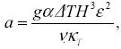and saline 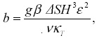Rayleigh numbers, the Lewis number or diffusivity ratio the Prandtl number and the aspect ratio or wave number

We used the following standard case parameters (SCP): L = 50 cm, H = 6 cm, ΔT = 20 °C, ΔS=9‰, q = 2×0.8 cc/s. Thus, the principal 2-D model parameters in the present series of experiments could be evaluated as a = b = 2×10⁷, ε = 0.37, Le = 10^-2, Pr = 10. These parameter values are in the space of control parameters analysed previously by Cessi and Young (1992), Quon and Ghil (1992), Thual and McWilliams (1992) with the exception of the Lewis number which was accepted at one or two magnitudes greater in the numerical calculations.

Two more dimensionless parameters could be useful to quantify the convectively driven flows. Thus, the stability of homogeneous flows is determined by the value of Reynolds number

where U is the scale of the horizontal velocity. The transition of laminar homogeneous flow to the turbulence occurs when this parameter exceeds the critical value (Re>2000). For the stratified case, a flow has a density distribution in a vertical direction. At the boundary of 2-layer flows, internal waves occur. The stability of internal waves and turbulence depends on the Richardson number:

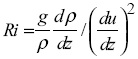
For small Ri values less than critical value (approximately 1/4), the internal waves become unstable. This leads to the mixing of the two fluids, breaking their interface due to Kelvin-Helmholtz instability and transition to the turbulence.

 

3. Experimental results

The following series of laboratory experiments was carried out to test any assumptions proposed, and results obtained in the theoretical models. The related questions are: (1) what are the differences (qualitative and/or quantitative) in thermally and haline driven circulation; (2) what are the special features of doubly driven flows in laboratory conditions.

Before proceeding with the study of the flows in a two-component fluid, the experiments exclusively involving temperature or salinity forcing were performed first. Initially, a set of laboratory runs was generated to quantify the intensity of the thermally and haline driven motion in the present model configuration. In Stommel's model, the water volume flux between two interconnected basins subjected to salt and temperature influences is considered to be linearly related to the density difference difference (Q = cΔρ). To test this theoretical assumption, laboratory experiments were conducted for a number of values of temperature (0 <ΔT < 50 °C) and salinity (0 < ΔS <12%) differences between the polar and equator boxes imposed from the bottom (partial convection regime (II)). The curves of maximum velocities observed for the steady states are shown in figures 5a, b versus temperature and salinity differences. As is visible from the measured data, thermally driven motion was more intensive in comparison to haline driven circulation. For example, for the SCP (ΔT = 20 °C and ΔS = 9%), density differences had approximately the same values Ap/p = 6.7x10^Q, but the velocity of thermally driven circulation was approximately 9 times higher (0.70 cm/s versus 0.075 cm/s). One of the probable reasons is that temperature and salinity have an opposing influence on the kinematic viscosity of seawater.

It usually takes 1 hour for thermally or about 3 hours for salinity driven experiments to reach the steady state. Therefore, δ = 1/3 could be estimated for our laboratory runs. The thermally driven experiments with different combinations of boundary conditions at the top and bottom boundaries have shown that the maximum velocities were generated in the maximum convection regime (IV) (up to 0.85 cm/s for the same values AT = 20 °C and other SCP), and correspondingly, the minimum values (less than 0.20 cm/s) were measured in the minimum convection regime (I).

The scale of velocity for convectively driven flows could be evaluated based on the ratio of buoyancy force to inertia Co=Gr/Re², where

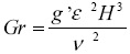
is the Grashof number, which, in turn, is the ratio of the Rayleigh number to the Prandtl number. When the buoyancy force and inertia are both of the same value, it follows that U~ε(g'H)^1/2. The theoretical curve

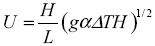
is shown in Figure 5c in comparison to the experimental data (Fig. 5a). These graphs illustrate that a relationship between external forcing and internal dynamics was close to a "1/2" fractional law in laboratory conditions.

In previously cited 2-D theoretical models, one of the principal model parameters was defined specifically as Le = 1 or/and 0.1. These settings allow for elimination of certain computational difficulties associated with a very small diffusivity, such as having to use extremely small time steps (see discussion in Quon and Ghil, 1992). In contrast, Schmitt (1994) reported that for ocean conditions there are two orders of magnitude difference in heat and salt diffusivities (Le = 10^-2). Therefore, it was important to understand which is the order of the Lewis number in laboratory conditions. An analysis of the vertical structure of the temperature and salinity driven circulation could serve this purpose.

The experiments (I)-(IV) with combination of boundary conditions at different elevations have shown that temperature driven circulation in all these runs for the SCP (H = 6 cm) had a symmetrical 2-layer structure with surface water moving from the equator to the pole box (Fig. 6a). Such kinds of 1-cell motion with water descending at the polar box and rising at the equator box were reported practically in all theoretical models.

Analogous experiments with only salinity forcing have shown that for the same SCP, the vertical structure of circulation was different for boundary conditions differently imposed at the vertical boundaries. Thus, S-driven circulation was symmetrical 2-layer with surface flow directed from the pole to equator box for the maximum convection regime (IV) (Fig. 7a). Under the surface forcing (i.e. for the partial convection regime (III)), the S-driven circulation was an asymmetrical 2-layer concentrated at the upper half of the plane with almost stagnant water near the bottom (not shown). At least a 4-layer symmetrical circulation with formation of secondary flows at mid depths was formed for the minimum convection regime (I) (Fig. 7b).

This layered structure of circulation in the minimum convection regime (I) primarily consists of flows at the diffusive boundary layers and opposing secondary flows in the channel interior. Diffusion appears to produce the primary flows near the vertical boundaries at the layers of diffusivity (h), whereas the formation of secondary flows at mid depths at layers (μ) results from flow viscosity. The same structure was observed in the partial convection regime (II) as well; however, not observed in the partial convection regime (III). A possible reason is that all the buoyancy energy produced under the bottom forcing is supplied by gravity that moves salt downward. This produced a more sluggish motion in comparison to the surface forcing experiment, and thus, a greater viscous layer.

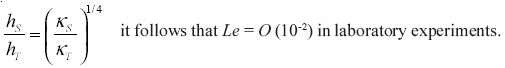
The vertical scale of layers of diffusivity as stated by Quon and Ghil (1992) is proportional to the Rayleigh number (h~Ra^-1/4) or to the coefficient of diffusivity (h~k^1/4). As visible from Figure 7b, the width of a layer of salt diffusivity at the channel center for the chosen SCP is about h_s = 1 cm. The vertical scale of the layer of viscosity (μ= v/w) is a measure of the distance over which the vertical advection is damped through viscous friction. In this viscous layer located in the channel interior, the pressure gradient could change the sign (see Fig. 8.26 from Potter and Wiggert, 1998). In such a case, an unfavorable pressure gradient causes secondary flows at mid depths.

A similar formation of layers of viscosity, and a 4-layer structure of circulation, have been seen in the thermally driven minimum convection regime (I) for increased water depth (H = 15 cm) and other SCP (Fig. 6b). Here, the layer of heat diffusivity at the channel's center was approximately h_T = 3 cm. As thermal and saline Rayleigh numbers were equal, and as the layer of heat diffusivity was approximately 3 times greater than the layer of salt diffusivity, from

Finally, a series of laboratory runs was conducted to understand the characteristics of the doubly T-S driven flows with different combinations of boundary conditions at the top and bottom boundaries. An essential finding from these experiments is that a primarily layered structure of THC and a collection of hybrid steady states were observed for the SCP, which was not noted by the earlier theoretical models.

Minimum convection or double diffusion regime (I). Let us first consider the flow patterns observed for the double diffusion regime with an absent convection. In this regime, after a few running hours (usually it takes 3-4 hours to reach the steady state for the SCP in the doubly driven experiments), the THC was observed as a quasi-symmetrical 3-layer system with the surface and bottom flows directed from the equator to the pole box. The sketch of the measured velocity and a corresponding photograph are shown in Figure 8a and Figure 9a accordingly. The formation of these flow patterns could be understood in the following manner. From previous experiments, it is known that the layer of salt diffusivity is narrow enough (h_s≈ 1 cm) for the SCP. Thus, salt-water is concentrated near the bottom layer, whereas the fresh water is disposed above. As a result, a 2-cell circulation is realized in the vertical plane. That is, a bottom cell is salinity driven, and a top cell is thermally driven.

Measuring of the sample salinity (or density ρ_s using densimeter at a constant temperature) and the temperature at discrete levels (which was converted to density ρ_T = ρ_g(l-aT) using Anton Paar tables was carried out in these experiments. The resulting density profiles are shown in Figure 8a as well. They illustrate a stable temperature and salinity distribution in the vertical. The hydrological and circulation patterns for such a kind of experiments are characterized by the relatively low Reynolds

Partial convection regime (II). The flow patterns observed in this regime under the bottom forcing were similar to those previously discussed for the minimum convection regime, i.e. 3-layer system of circulation with a slightly greater Reynolds number (Re = 195). The distinctive feature is that instabilities of the Kelvin-Helrnholtz type were realized at the sharp boundary separating mid depth and bottom flows (Fig. 9b). As can be seen from Figure 8b, temperature distribution was unstable with the minimum value measured at mid depth (Ri_T = -2 for the lower semiplane), whereas a stable solute distribution (Ri_s = 28) compensated for this unstable temperature profile. Thus, warm salty water near the bottom was set beneath cold fresh water at mid depth. As noted by Stern (I960), when this water is displaced upward from below, it loses the heat and causes the restoring oscillations and instabilities. This "salt fountain" effect was neglected in Stommel's model supposing that lighter water is only able to float on top of the denser deep water.

Partial convection regime (III). For this regime (surface forcing) we observed a reversed 3-layer circulation approximately of the same intensity (Re = 190), but with the surface flow directed from the pole to the equator box (Fig. 8c) and with the Kelvin-Helmholtz instabilities localized between surface and subsurface flows (Fig. 9c). The hydrological structure was opposite to the previously discussed case as well. Here, the temperature profile was unstable, showing the maximum temperature values at mid depth (Ri_T = -7 for the upper semiplane). The salinity profile was stable (Ri_S = 27) there, with the sharp halocline formed near the surface. In such a case, the salty warm water descends from the surface to the bottom due to convection. This descent releases heat, but not salt, to surrounding water. The downwelling from the surface near the equator box yields surface circulation directed from the pole to the equator. This surface current has the characteristics of polar water. As a result, the 3-layer hydrological structure there (cold and fresh water in the upper layer, warm and salt-water at mid depth, cold and salt-water near the bottom) forms the corresponding 3-layer system of currents.

Maximum convection regime (IV) revealed that circulation also has a 3-layer structure (Fig. 8d) typical for the double diffusion (I) and for the partial convection (II) regimes. The characteristic feature of water movement in this experiment was a realized regime of increased turbulence (Fig. 9d). These circulation patterns were accompanied by unstable temperature as well as salinity profiles (Fig. 8d) showing the colder, fresher water at mid depths.

These doubly driven experiments (I)-(IV) illustrate the well-known fact that thermal and salinity driven circulations are not additive due to strong non-linearity in the heat and salt advection. A few more experiments were conducted to understand how the aspect ratio parameter, a wider range of the buoyancy ratio, and an increased mixing, affect the circulation patterns. In these experiments we just analyzed the flow structure.

The experiments with water depth variance have shown that the aspect ratio parameter controls the number of layers of the doubly driven flows as well. For example, the formation of additional layers of circulation was obvious in the experiments with an increased water depth. That is, a 5-layer circulation was realized in the maximum convection regime (IV) when H = 15 cm (not shown), whereas the 3-layer circulation noted previously was kept when H = 3 cm. Experiments with a more shallow water depth were not conducted in this series of laboratory runs.

Experiments with a wider range of the external forcing parameter (R) were carried out in the following manner. We started each experiment for the minimum water depth (ε = 0.18) with initially rested and homogeneous salt-water (4.5‰) at room temperature. Salinity difference (ΔS = 9‰) between the pole and the equator boxes was kept constant. The pole box temperature was always T_p = 20 °C, whereas the temperature in the equator box was changed (25° < T_e< 60 °C) slowly and regularly (about 1°C every 20 minutes). In such a case, the buoyancy ratio was changed as 0.5 < R < 4. These experiments were conducted for the equator box temperature both being slowly increased and decreased from the extreme interval values. These were carried out for the differently imposed boundary conditions at the vertical boundaries as well. Thus, eight experiments went into this Figure including four different regimes of circulation I-IV with equator box temperature both being slowly increased and decreased. The results for the series of laboratory runs are summarized in Figure 10.

These experiments have confirmed the existence of the 3 steady states for the defined interval of the forcing parameter: 2-layer T-mode circulation (T2) when R < 0.7, 2-layer S-mode of water motion (S2) when R > 1.6 and 3-layer hybrid state (H3) when 0.9 < R < 1.2. Transition between thermal and hybrid states (TH-transition) was realized for 0.7 < R < 0.9, and transition between hybrid and saline states (HS-transition) occurred for 1.2 < R <1.6. The HS-transition is shown in Figure 11a, b, c. This result is relatively novel, as the previous laboratory experiments by Whitehead (1996, 1998) and Whitehead et al. (2003) reported just existence of T2-H3 transitions.

Transition of the 3-layer hybrid state to the 2-layer circulation was seen as suppression of the surface or bottom flow. As is visible from Figures 5a, c, the temperature changes of about 10 °C from the SCP (ΔT = 20 °C) are needed to suppress the flow of the 0.25 cm/s intensity. The T2-H3 and H3-S2 transitions in these natural convection experiments were always smooth. Though the maximum and partial convection regimes produced Kelvin-Helmoholtz instabilities as noted previously, its own energy was not sufficient for inducing abrupt transitions. On the contrary, abrupt transitions and flow oscillations were observed during several experiments with an increased mixing within TH and HS intervals. Additional mixing was generated by two mixers installed in the polar and the equator boxes. Their rotation rate was -200 rpm (revolutions per minute). A complete mixing produced small stratification in the test channel and allowed flow to overcome the damping effect of the layered structure. The abrupt transitions appeared both in a dye visualization and in density records. Theoretically predicted direct transitions between T2 and S2 states were not observed here, probably because of the different Lewis numbers in the numerical calculations and in our experiments. These complete mixing experiments are supposed to be continued in a further study.

 

4. Discussion and conclusions

Stommel's theory predicted the multiplicity of thermohaline circulation in the hydrodynamic systems for the defined conditions. In this model, two boxes were filled with well-mixed water and subjected to the temperature/salinity influences through side walls. A key element of the Stommel's theory is the postulate law (3), where transport is linearly proportional to density difference. Due to the box model constraints, the Stommel's scheme of THC was a 2-layered one with heavy water flowing under light water. The two modes of circulation (T- and S-states) were predicted in this box model. Necessary and sufficient conditions for multiple equilibria were found by Stommel (1961) in the form of (4)-(5).

Further theoretical studies of the present problem using 2-D models were carried out by Marotzke et al. (1988), Cessi and Young (1992), Quon and Ghil (1992), Thual and McWilliams (1992). According to the 2-D theory results, mixed boundary conditions (prescribed temperature and salt flux condition) at the vertical boundaries could produce multiple equilibria of the THC. Their studies have illustrated that at least four model parameters, thermal (a) and saline (b) Rayleigh numbers (or the buoyancy ratio R = b/a), Lewis number (Le), and aspect ratio (ε), should control multiple solutions. The 1-cell thermally driven and 1-cell salinity driven water motions were described as possible modes of circulation in these 2-D models for the pole-equator system. The existence of the additional hybrid states was predicted for the pole-to-pole circulation for the defined range of the control parameters.

Laboratory experiments by Whitehead (1996, 1998) and Whitehead et al. (2003) were the first to illustrate that multiplicity of THC is not only a mathematical problem of the multiple solutions under the mixed boundary conditions, but a real hydrodynamic problem of different flow structures. The multiple states were found in the 1-box chamber (heated from below and subjected to increased salinity from above), i.e. in the maximum convection experiments. This chamber was connected to the well-mixed external reservoir. Equilibria was observed here between 2-layer (T2) and 3-layer (H3) flow systems in the space of the control parameters (R-1, δ-1/3 and ε -1). Whitehead et al. (2003) reported that depth of salt-water intrusion (or rate of the mixing) greatly affects the multiple equilibria as well.

The present series of laboratory experiments were carried out to test the principal assumptions and theoretical results proposed by Stommel (1961). Presently, we would like to test the postulate law (3) to verify the necessary and sufficient conditions (4)-(5) of multiple equilibria; to understand the role of the "well-mixed water" condition, and of boundary conditions at different elevations in the phenomena. The main goal of the present laboratory experiments is to clarify the question of whether the transitions are abrupt in Stommel's thermohaline box model.

A new apparatus was designed for investigating this problem. In the new model constraint, two water basins (equator and pole boxes) were connected by a rectangular channel representing an oceanic basin. The flow field there was generated by a double temperature/salinity forcing. The equator box was heated and subjected to salt-water intrusion. The pole box was cooled and affected by the fresh water flux. The boundary conditions at different elevations produced maximum convection, partial mixing or double diffusion regimes in the boxes. Thus, the condition of the "well-mixed water" was replaced here by natural convection and diffusion processes.

First of all, the relative strength between external forcing and internal dynamics (3) was quantified in a series of thermally and salinity driven experiments. The results of the laboratory runs have shown that the relationship between volume transport and density difference is close to the "1/2" fractional law in laboratory conditions. As visible from Figure 6 in Stommel (1961), such kinds of curve replacement should not alter the general conclusions of the Stommel's multiple states theory.

Nilsson and Walin (2001) showed recently that this relationship between the strength of the circulation and the density difference can change from direct, as assumed by Stommel (1961), and supported by our experiments, to inverse under some assumptions about the diapycnal mixing in the ocean. For example, as it is shown, the inverse dependence occurs if one assumes that the coefficient of diapycnal mixing is inversely proportional to the buoyancy frequency.

The second issue of the laboratory study centered on which steady states of the THC could be realized in the experiments with double temperature/salinity forcing. The earlier box model and 2D theory both predicted 1-cell thermally or 1-cell salinity driven circulation in the vertical plane of the pole-equator system. We have found that THC could be more complicated, as three steady states were found for the doubly driven experiments in the range of the forcing parameters. These are 2-layer thermal (T2), 2-layer saline (S2) and 3-layer hybrid state (H3) separating two 1-cell modes of water motion in the space of a control parameter (R). These hybrid states were observed in experiments I-IV with the boundary conditions at different elevations when the buoyancy ratio was close to unity (0.9 < R < 1.2).

A probable reason why the experiments and theory differ is that Stommel (1961) presumed beforehand formation of the 2-layer circulation in his model constrain (two boxes connected by two tubes at the top and bottom). As far as we can determine, 2-D theoretical models have not reported existence of the hybrid state (H3), because of the different Lewis numbers in the numerical calculations and in the laboratory runs. The dynamics in the laboratory experiments are very much controlled by the small diffusivity ratio (Le = 10^-2). Hence, the large Le number argument is no longer valid. Quon and Ghil (1992) noted that decreasing value of this parameter influences a tighter packing of the isolines, i.e. it is responsible for producing a layered structure of the circulation. We speculated that following theoretical studies should pay attention to this experimental result. In such a case, the possible different stability curves and the criteria of multiple equilibria could be obtained.

The other point of disagreement between the theory and the experiments is the stability of THC. In Stommel's conceptual model, the heavier liquid flows below the light one. Our experiments show that it is not always the case. Thus, in the maximum convection and in the partial mixing experiments, water of greater density penetrates the mid depth. In its turn, it is favorable to cause instability of the Kelvin-Helmholtz type. As in the natural convection experiments, we always observed the smooth TH and HS transitions; this means that energy of these instabilities is not sufficient for abrupt Stommel's transitions.

The Stommel's theory predicted that multiple equilibria should be realized for 1< R < 3 if δ~1/3 (estimated for the laboratory conditions), when X is a small enough parameter. The present laboratory experiments were conducted for the space of control parameters needed for this phenomena. When we followed an experimental path in the control space, i.e. slowly varying temperature of the equator box and fixing all the other parameters, circulation exhibited smooth transitions for natural convection experiments within TH and HS intervals (see regime diagram in Fig. 10). The abrupt changes in flow direction and speed, a feature that is referred to as a Stommel's transitions, were not present at all.

An appearance of the Stommel's transitions was only found in the present laboratory runs when polar and/or equator boxes were stirred with the use of mixers. An additional mixing increases instability effects causing the indifferent stratification and a possibility of the abrupt transitions. As previously, multiple states and Stommel's transitions were found in the laboratory just for well-mixed water experiments (Whitehead, 1996, 1998; Whitehead et al., 2003), we suppose this to be a necessary condition for this phenomena. These results are not in disagreement with the Stommel (1961) assumption that water in the boxes should be well mixed.

The following question arises: How do complete mixing experiments relate to the real ocean? We suppose that in the sea-water basins many sources of mixing contribute to providing a condition of well-mixed water. These include turbulence, winds and tides driving and breaking internal waves.

In the present complete mixing experiments, Stommel's transitions were found to be two-fold: H3-S2 and T2-H3 transitions of flows, even though the Stommel's theory predicted direct transitions between thermal and saline modes of THC. This turns to be one of the principal findings of the present series of laboratory runs, as previously Whitehead et al. (2003) reported only T2 and H3 transitions.

Thus, we have not received a one-to-one correspondence between Stommel's theory and laboratory experiments in detail. Nevertheless, if we try to answer the principal question of whether the transitions are abrupt in Stommel's thermohaline box model, we can say, that they could be. However, the condition of "well-mixed water" is crucial for this phenomenon to occur.

 

Acknowledgements

The present study was funded by CONACyT (Mexico) for project 32499-T. Dr. J.A. Whitehead was responsible for creating the authors interest in the problem. We appreciate the effort by Gary Gaje who helped with the English grammar. We gratefully acknowledge the constructive comments of two reviewers who helped improve the content and presentation of this paper.

 

References

Anton Paar, 2000. Instruction handbook for density/specific/concentration meter DMA 4500/ 5000. Graz. Austria. Document number XDLIB07EP65, 108 p.         [ Links ]

Bryan, E, 1986. High-latitude salinity effects and interhemispheric thermohaline circulations. Nature 323,301-304.         [ Links ]

Cessi, P. and W. R. Young, , 1992. Multiple equilibria in two-dimensional thermohaline circulation. J. Fluid Mech. 241, 291-309.         [ Links ]

Dijkstra, H.A. and M.J. Molemaker, 1997. Symmetry breaking and overturning oscillations in thermohaline-driven flows. J. Fluid Mech. 331, 169-198.         [ Links ]

Manabe, S. and R. J. Stouffer, 1988. Two stable equilibria of a coupled ocean-atmosphere model. Climate Dyn. 1, 841-866.         [ Links ]

Marotzke J., P. Welander, and J. Willebrandt, 1988. Instability and multiple steady states in a meridional-plan model of the thermohaline circulation. Tellus 40A, 162-172.         [ Links ]

Marotzke, J., 1993. Ocean models in climate problems. In: Ocean Processes in Climate Dynamics: Global and Mediterranean examples (Malanotte-Rizzoli, P. and Robinson, A.R., eds.), Kluwer Publ., 79-109.         [ Links ]

Nilsson, J. and G. Walin, 2001. Freshwater forcing as a booster of thermohaline circulation. Tellus 53A, 629-641.         [ Links ]

Potter, M.C. and D.C. Wiggert, 1998. Mechanics of Fluids, 2^nd ed., Prentice Hall, 776 p.         [ Links ]

Quon, C. and M. Ghil, 1992. Multiple equilibria in thermosolutal convection due to salt-flux boundary conditions. J. Fluid Mech. 245, 449-484.         [ Links ]

Quon, C. and M. Ghil, 1995. Multiple equilibria and stable oscillacions in thermosolutal convection at small aspect ratio. J. Fluid Mech. 291, 33-56.         [ Links ]

Rooth, C., 1982. Hydrology and ocean circulation. Progress in Oceanography 11, 131-149.         [ Links ]

Ruddick, B. and L. Zhang, 1996. Qualitative behaviour and nonoscillations of Stommel's thermohaline box model. J. Climate 9, 2768-2777.         [ Links ]

Schmitt, R. W., 1994. Double diffusion in oceanography. Ann. Rev. Fluid Mech. 26, 255-285.         [ Links ]

Stern, M.E., 1960. The "salt fountain" and thermohaline convection. Tellus 12, 172-175.         [ Links ]

Stommel, H. and A. B. Arons, 1960. On the abyssal circulation of the World ocean. 1. Stationary planetary flow patterns on a sphere. Deep-Sea Res. 6, 140-154.         [ Links ]

Stommel, H., 1961. Thermohaline convection with two stable regimes of flow. Tellus 13, 224-230.         [ Links ]

Straub, D. N., 1996. An inconsistency between two classical models of the ocean buoyancy driven circulation. Tellus 48A, 477-481.         [ Links ]

Thual, O. and J. C. McWilliams, 1992. The catastrophe structure of thermohaline convection in a two-dimensional fluid model and a comparison with low-order box models. Geophys. Astrophys. Fluid Dyn. 64, 67-95.         [ Links ]

Welander, P., 1982. A simple heat-salt oscillator. Dyn. Atmos. Oceans 6, 233-242.         [ Links ]

Whitehead, J. A., 1995. Thermohaline ocean processes and models. Ann. Rev. Fluid Mech. 27, 89-113.         [ Links ]

Whitehead, J. A., 1996. Multiple states in doubly driven flow. Physica h 97, 311-321.         [ Links ]

Whitehead, J. A., 1998. Multiple T-S states for estuaries, shelves, and marginal seas. Estuaries 21(2), 281-293.         [ Links ]

Whitehead, J. A., M. L. Timmermans, W. G. Lawson, S. N. Bulgakov, A. Z. Martinez, J. M. Almaguer, and J. Salzig, 2003. Laboratory studies of a thermally and/or salinity driven flows with partial mixing. Part 1: Stommel transitions and multiple flow states. J. Geophys. Res.-Oceans 108(C2), 3036-3052.         [ Links ]

Winton, M. and E.S. Sarachik, 1993. Thermohaline oscillations induced by strong steady salinity forcing of ocean general circulation models. J. Phys. Ocean. 23, 1389-1410.         [ Links ]