Sensitivity of a two-dimensional convective model to turbulence parameterization

 

MATILDE NICOLINI and MARCELA TORRES BRIZUELA

Departamento de Ciencias de la Atmósfera y los Océanos, Universidad de Buenos Aires, Centro de Investigaciones del Mar y la Atmósfera (UBA-CONICET), Buenos Aires, Argentina

 

(Manuscript received March 19, 2001; accepted in final form Dec. 3, 2001)

 

RESUMEN

Se investiga la sensibilidad de un modelo bidimensional con una mejora en la parametrización de la turbulencia. Este modelo (de ahora en adelante Modelo de la Universidad de Buenos Aires, UBA) es capaz de simular un escenario factible de la convección en un caso real, caracterizado por fuertes vientos divergentes observados en superficie. Las principales mejoras han sido hechas en el tratamiento de la turbulencia para el modelo con microfísica correspondiente a la fase mixta utilizando un cierre de la turbulencia de primer orden. Con el fin de cumplimentar este objetivo se realizaron cuatro experimentos numéricos.

Los resultados muestran que la nueva parametrización de la turbulencia afecta la simulación de la convección. El énfasis del trabajo está puesto en la representación de una de las características más significativas del evento convectivo usado en este test de sensibilidad. La velocidad máxima del viento en superficie correspondiente a la ráfaga en la descendente más intensa es mejor aproximada por la representación de un K_m variable.

A fin de documentar si la sensibilidad del modelo UBA es una característica peculiar del mismo se usó el Advanced Regional Prediction System (ARPS) para contrastar los resultados del modelo UBA. El modelo ARPS muestra una mayor sensibilidad a la turbulencia.

En comparación con todos los experimentos bidimensionales, la inclusión de la tercera dimensión refuerza el movimiento vertical pero reduce los flujos divergentes en superficie. El desempeño del modelo UBA resulta ser superior a la versión ARPS-2D en términos de la intensidad de los flujos divergentes en superficie provenientes de la convección para el caso de la tormenta en el aeropuerto de Resistencia. Este resultado es prometedor y justifica validar en el futuro el modelo UBA en otros casos de vientos intensos divergentes en superficie a modo de mejorar su capacidad como herramienta de pronóstico en aeropuertos.

 

ABSTRACT

The sensitivity of a bidimensional cloud model with an upgraded turbulence parameterization is tested. This model, denoted as University of Buenos Aires model (UBA) has the ability to simulate a credible convective scenario in a real data case characterized by observed strong outflows. The main improvements have been made over the turbulence parameterization for the mixed phase microphysics using a first order turbulence closure. Four experiments were performed to accomplish this objective.

Results show that the new turbulence parameterization affects the simulation of convection. The emphasis is in the representation of one of the significant features of the convective event used in this sensitivity test. Maximum surface wind speed corresponding to the strongest downdraft is better approached by the representation of a variable K_m.

In order to find out whether the sensitivity of the UBA model to the turbulence parameterization is a peculiar characteristic of this model, the Advanced Regional Prediction System (ARPS) was also implemented to check results from the UBA model. ARPS model also shows sensitivity to the turbulence parameterization with a stronger impact.

Compared with all 2-D experiments, the inclusion of the third dimension enhances the vertical motions but reduces the divergent outflows at the surface. The UBA model performance proves to be higher than the ARPS 2-D version in terms of convective outflow strength near the surface in this simulated case, at Resistencia airport. This result is encouraging and justifies future validation of the UBA model in other downburst cases in order to asses its capability as a prognostic tool in airport forecast activities.

Key words: Convection, turbulence parameterization, modeling.

 

1. Introduction

Numerical simulation of convection has been the focus of many studies since the pioneer work of Malkus and Witt (1959). Among the several articles on this subject are those of Klemp and Wilhelmson (1978), Clark (1979), and books like those by Cotton and Anthes (1989) and Emanuel (1994).

Models are frequently viewed as a tool for further understanding of convective processes and in particular of mechanisms related to connectively driven weather phenomena. The study of such phenomena is not only of theoretical interest. A better understanding of different mechanisms acting within convective clouds allows very short-term forecast of these severe events in support to aviation. Nicolini and Torres Brizuela (1997) documented the occurrence of surface strong winds related to convection at Ezeiza and Resistencia airports in Argentina during the 1959-1979 period. Analysis of this sample revealed that around 350 days verified the imposed criterion for qualifying as severe winds at both airports.

Concern about the fact that available computers at airports are not fast enough to run 3D versions of models to predict these phenomena with sufficient time to improve the security at the airport terminals has motivated the use of 2D models as an alternative tool. Proctor (1989), Tuttle et al. (1989) simulated the intensity of convective down drafts with two-dimensional models obtaining positive results.

Lack of well-documented observations during storms in Argentina prevents a detailed comparison of simulated against real down burst phenomena. Also, such a detailed comparison is too stringent a test for a 2D model with a microphysical parameterization that is currently being improved (Carrió and Nicolini, 1999, Carrió and Nicolini, 2000). Therefore, a 2-D model performance is tested and related to the reproduction of winds at least as strong as the observed maximum surface wind speed at airports in a particular convective case.

A two-dimensional convective model has been developed at the University of Buenos Aires (Nicolini, 1986; Nicolini and Paegle, 1989). This model (UBA) has been tested in a well-documented storm generating a "wet microburst" observed over Alabama, USA (Nicolini, 1993) and used to demonstrate the benefits of higher model resolution in predicting extreme rainfall events (Nicolini et al., 1993). The version used in these papers included a turbulence parameterization with a constant eddy diffusion coefficient. An examination of the results and a review of the observations in Nicolini (1993) showed that the cloud evolution and the microphysical processes satisfactorily matched reality. The maximum differential radial velocities over the microburst observed and its horizontal extent were well captured by the model. However, the precipitation collapse rate and horizontal cloud dimensions were not simulated equally well.

It has been known that turbulence is crucial to the successful simulation of small-scale atmospheric convection ϒ scale according to Orlanski, 1975). The problem of parameterizing turbulent fluxes on numerical models in a realistic and feasible way according to computational facilities is still subject to discussion. Clark (1979) provides adequate background for using the first order closure in deep convection. He discovered that in this type of convection, turbulent kinetic energy is smaller than that solved by the model. This result is very important because in three-dimensional deep convective models, the grid length is usually (≈ 500 m) out of the inertial subrange. Uliasz (1994) reviewed the problem of turbulence parameterization from the first to higher order closure theories. As Uliasz explained, third order closure on mesoscale models has been limited to a few idealized situations and has been used in few cases over the convective scale (Krueger, 1988).

A correct representation of entrainment is supposed more crucial in shallow than in deep convection and then first order closure is assumed sufficient for many applications of a deep convective model. The UBA model with the inclusion of this type of turbulence parameterization was applied by Nicolini and Torres Brizuela (1997) to study the contribution of different downburst forcings in a downburst-producing storm in Resistencia, Argentina. Nicolini and Torres Brizuela (1999) describe the theoretical background of the upgraded version of the model.

The main purpose of this study is to test the sensitivity of the UBA model to the inclusion of a non-constant in time and space eddy diffusion coefficient. In order to find out whether the sensitivity of the UBA model to the turbulence parameterization is a peculiar characteristic of this model, it has been tested against a state-of-the-art convective numerical model. The model used is the Advanced Regional Prediction System (ARPS), developed by the University of Oklahoma (Xue et al., 1995). This model has been already tested in several situations and allows the inclusion of a higher order turbulence parameterization.

The UBA convective model and the formulation of the first order turbulence closure are briefly described in section 2 of this paper. The study case description and the characteristics of the sensitivity experiments are included in section 3. The results are presented in section 4 and the conclusions are summarized in section 5.

 

2. Models Description

2.1. UBA Model

The UBA two-dimensional deep convective model uses the anelastic approximation according to Lipps and Hemler (1982). Motion is supposed to be confined to a vertical plane. Both characteristic time scale and Rossby number for non-organized convection allow neglection of Coriolis terms in the governing equations (Emanuel, 1986). Also, through scale analysis viscous terms are ignored.

The set of equations include a prognostic equation for vorticity in the x-z plane, a thermodynamic equation and prognostic equations for specific humidities for different water categories. Water categories include: water vapor (q_v), cloud droplets (q_c), rain droplets (q_r), cloud ice (q¡), snow (q_s) and graupel/hail (q_g). The microphysical parameterization follows a bulk water formulation (Lin et al., 1983; Lord et al., 1984). The basic microphysical processes included are: evaporation of rain, melting and sublimation of snow and graupel, Bergeron processes which transform water and cloud ice into snow, autoconversion of suspended particles into precipitating particles and the accretion between each precipitating category and other liquid and solid categories. The procedure used to compute the total production terms, depends on whether the temperature is above or below 0°C.

The closure for the set of equations uses K-theory. Formulation of the momentum diffusion coefficient K_m assumes an equilibrium value for the turbulent kinetic energy through a balance among the shear mechanical production, the buoyant production due to the existence of a turbulent heat flux diminished by the load of hydrometeors and the energy dissipation by viscosity forces (ε). K_m and ε are modeled according to diagnostic equations following Mellor and Yamada (1974). The derived expression for K_m results:

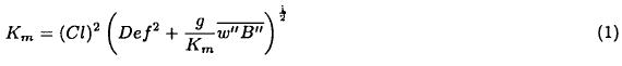
where C is an arbitrary empirical constant, l is the turbulent length scale assumed to be equal to (Δx.Δz)^1/2 (Lilly, 1967). Δx and Δz are the horizontal and vertical grid intervals, respectively. Def² is defined as:

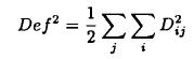
where D_ij is the mean rate of deformation tensor. Bars over individual variables refer to the mean value, primed variables identify deviations from the base state, which is supposed to be in hydrostatic equilibrium and is represented by the subindex zero.

is the buoyant subgrid scale flux term where the expression for buoyancy B' is:

where q'_v and q'_t represent the deviations of water vapor and total condensed water from the base state values.

Potential temperature deviation is denoted by θ' and θ₀ is the base state potential temperature.

Nicolini and Torres Brizuela (1999) derived the expression for K_m (1) for three different air cases: only liquid phase (non-saturated moist, saturated moist air) and mixed phase microphysics including ice.

In the non-saturated moist air case the derived expression for K_m is

whereas for the saturated moist air case it becomes

where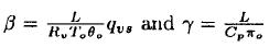

θ_v is the virtual potential temperature and the coefficient K_h is related to K_m through the Prandtl number (P_r)

P_r is assumed to be equal to 1, according to Clark (1979) and Tag et al. (1979).

Recalling the definition of the Brunt-Väisälä frequency following Emanuel (1994)

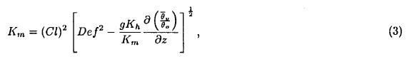
The expression for N² for a system composed by saturated air in the presence of liquid water is obtained replacing the expression for W"B" derived in Nicolini and Torres Brizuela (1999) in (6).

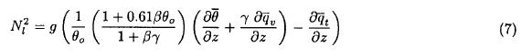
(7) a final form for K_m is

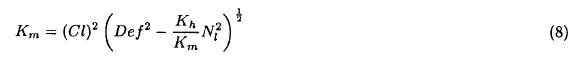
Durran and Klemp (1982) obtained an approximate expression of N_l² (their equation (36) similar to (7)). Since the numerical schemes used to solve the equations system produce pseudo-diffusion, which might be equivalent to include a reference K_m , the assumption of K_rn = 0 in case the radical in (8) is negative, is made.

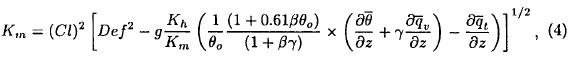
The complexity introduced by the ice phase in a microphysical treatment is due to the inclusion of terms, which represent parameterizations from the microphysics, and of a saturation adjustment. It is difficult to define a conservative thermodynamical variable as it was done for the liquid phase. Thus, the buoyancy frequency (6) for this case, is written as

and used in order to obtain an expression similar to (8) to calculate K_m for the general system that might be saturated in presence of water and/or ice. For mixed phase and in case of saturation we have

2.2. ARPS Model

The state-of-the-art numerical model used for intercomparison with the UBA model is the non-hydrostatic compressible ARPS model (Xue et al., 1995). Its microphysical parameterization and the included water species are similar to those used in the UBA model. It allows different options for the sub-grid turbulence processes: a first order subgrid scale (SGS) turbulence closure with constant eddy mixing coefficient, Smagorinsky-Lilly SGS diagnostic parameterization and a 1.5 turbulent kinetic energy closure.

 

3. Description of the initial conditions, numerical schemes, boundary conditions and experiments

A downburst-producing storm associated with a cold front occurred at Resistencia (27° 27' S, 59° 03' W), Argentina, on 23 October 1974 in the evening. This is one of the most severe cases included in the downburst statistics occurred at Ezeiza and Resistencia airports and relative contributions of different downburst forcings have been explored with the UBA model (Nicolini and Torres Brizuela, 1997). The convection generated intense downdrafts near the ground between 3 PM and 10 PM local time, and the observed maximum surface wind speed reached 24 m/s. The mean surface velocity during that period was 10 m/s. The Resistencia storm is characterized by a warm cloud base, a value of Convective Available Potential Energy of around 2207 m²s^-1, and approximately zero vertical shear, which justifies the decision to ignore it in the model simulations.

The two models used in this same case study were set up with the same domain, resolution and initial data, making model inter-comparison feasible and pertinent. Simulations with both models were initialized with the Resistencia sounding launched at 1200 UTC (Fig. 1), and with a bubble-like disturbance both in the potential temperature and the water vapor fields. This disturbance is located at the center of the domain, limited to the first 3.3 km and with an horizontal exponential intensity decrease from the maximum excess (1°C in θ and 2 g/kg in q_v). The integration domain is 39 km horizontal and 15.3 km vertical. The grid intervals in both horizontal and vertical direction are uniform and equal to 600 m whereas the time step is of 10 s. A staggered grid arrangement is used in both models.

As to the numerical schemes used in the UBA model, the advective terms, excluding the vorticity equation, are numerically treated using the Smolarkiewicz and Clark (1986) scheme, with one corrective step to reduce implicit diffusion. The corresponding terms in the vorticity equation are computed using the Arakawa (1966) scheme. Time derivatives in the vorticity equation are treated using the second order leapfrog scheme while the other prognostic variables are treated according to Smolarkiewicz and Clark (1986). To calculate K_m at the leading time level t + Δt, values at the middle level t of dynamical, thermodynamical and mixing ratios involved in (9) are used. K_m is defined at the same grid points as the ones where the thermodynamic variables are calculated. Turbulent terms are evaluated using the values for K_m and K_h calculated at t + Δt and the other variables are calculated at time t.

Regarding the UBA model boundary conditions, periodicity is assumed at the lateral boundaries unless otherwise specified. The use of these conditions restricts simulations to events characterized by an approximately zero vertical shear. Along the top and bottom of the model domain the velocity (w) is required to vanish, free slip conditions are assumed and the vertical gradient of the thermodynamic variables are set to zero. The condition for diffusive terms in the vorticity equation, is

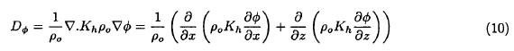
A similar assumption is made when we set the vertical gradient equal to zero for the diffusion term for any of the thermodynamic variables (ɸ) in the following expression

It is worth mentioning as a numerical difference with respect to the UBA model the inclusion in ARPS of a second-order computational mixing in the vertical, a fourth-order computational mixing in the horizontal and an Asselin time filter. This numerical smoothing is intended to damp small-scale numerical noise and to introduce a small amount of computational mixing even in stable regions where turbulent mixing is zero.

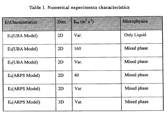
The main characteristics of the different experiments are listed in Table I. E₁ was performed to check the derived Brunt Väisälä frequency expression (7) against that obtained by Durran and Klemp (1982) for liquid-only microphysics. The remaining two experiments run with the mixed version of UBA model were conducted to test its sensitivity to the inclusion of the turbulence formulations proposed in the previous section for complete microphysics. The experiments performed with the ARPS model in a 2-D mode aimed at the exploration of the response of a model like the ARPS to similar turbulence alternatives. The ARPS model has also been run in a three-dimensional mode as a reference given the dimensional limitations of the UBA model. This 3-D ARPS version includes the more advanced unsteady turbulent energy equation (TKE) closure.

 

4. Results

Previous sensitivity experiments were carried out in a well-documented convective situation to determine the model's response to different values of the constant C (0.42, 0.2, 0.14 and 0.11) in the expression of K_m (equation 8). A C value equal to 0.11 is specified in the experiments E₁ to E₃, as this value gave the best results (not shown) for the maximum rising motion compared to observations (Wakimoto and Bringi, 1988).

In the E₁ case an analysis of the order of magnitude of N_m² has been done at strongest updraft time for saturated and non-saturated areas respectively. N_m² in unsaturated and stable areas over the top of the cloud attains positive values with a maximum of 2.7 x 10^-5s^-2. The same order of magnitude positive values are obtained within the first km near-neutral subcloud layer (maximum of 4 x 10^-5s^-2). N_m² in moist saturated unstable conditions attains negative values of around -2 x 10^-4s^-2 surrounding the updraft core. Negative values are also found up to the top of the cloud and in the first 2 km above the cloud base, whereas positive values of around 1.2 x 10^-4s^-2 characterize the updraft core. These values are lower or within the range given by Durran and Klemp (1982) in their comparison of different expressions for N_m² for two sets of temperatures and pressures for different environmental lapse rates. Their N_m² values range from -1.5 to 2.5 10^-4s^-2 in moist saturated conditions, and from 0.5 to 3.5 10^-4s^-2 in dry conditions.

Assuming that the treatment with a variable K_m and mixed microphysics is more rigorous, we first examined the results for the E₃ experiment.

During the Cu stage, convection develops until approximately 19 min, when the updraft reaches its maximum velocity of 30 m/s. Temporal evolution of the maximum values of specific humidity for the precipitating categories q_r, q_s, and q_g are displayed in Figure 2. In the simulated cloud, rain is started by coalescence, and later the processes linked to the solid phase are activated.

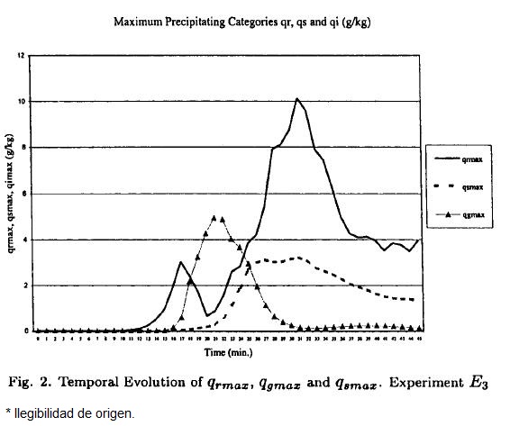
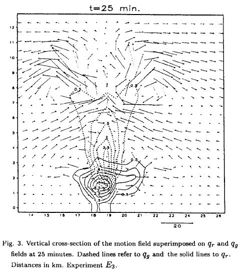
At about 21 min the graupel/hail category maximizes (5 g/kg, in Fig. 2) and two minutes later rainwater touches the ground. During the mature stage the cloud reaches its maximum top (13 km) and a downdraft, mainly forced by the precipitation loading related to q_r and q_g, and secondarily to evaporation of rain and melting of graupel (Nicolini and Torres Brizuela, 1997) is evident below 5 km in the motion field (Fig. 3, at 25 min). The q_g core, which has expanded both horizontally and vertically, extends below the melting level. The horizontal cloud dimension is around 7.5 km.

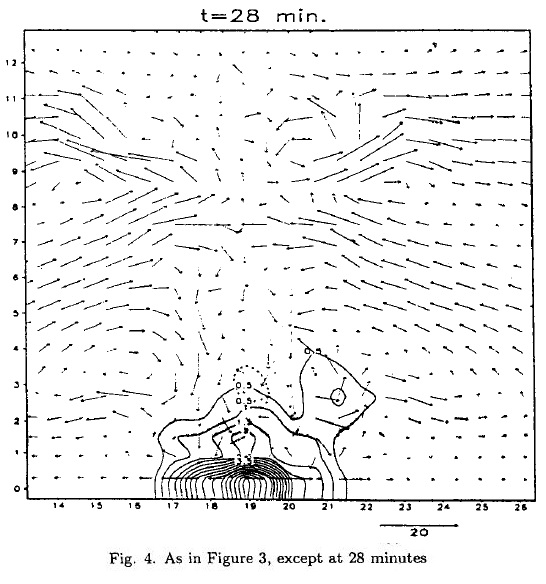
Dissipation stage is attained at around 28 min of integration time. Then, the q_r, q_g, and motion fields are depicted in Figure 4, the precipitation core reaches the ground (q_r = 8 g/kg) and ice and snow dominates from 7 to 13 km height. A maximum downdraft of-8 m/s is simulated at 600 m height and the u component field at the surface displays a peak differential horizontal velocity of 14 m/s in a distance of 1.8 km. If the maximum wind speed of 8 m/s is added to the environmental mean velocity of around 10 m/s, a maximum velocity of 18 m/s is obtained. This value underestimates the observed maximum surface wind speed of 24 m/s.

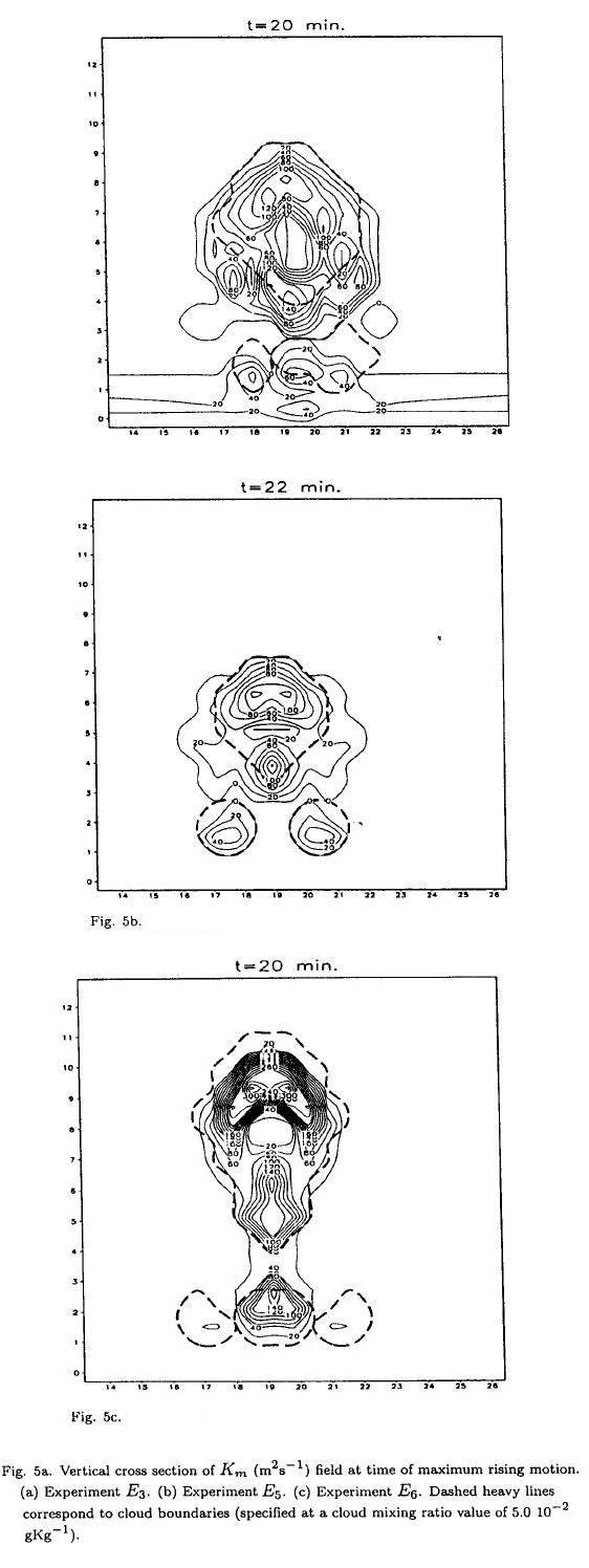
Consistent with the N_m², pattern, the K_m field at the time of maximum rising motion (see Fig. 5a) presents larger spatial variability in saturated areas. Maximum values (around 140 m² s^-1) are located where the moist instability is stronger above the buoyancy core, at the lateral boundaries, at the cloud base and within the upper part of the subcloud layer. A minimum (mostly zero value) is placed with the updraft core. K_m values different from zero are found in the unsaturated environment near the cloud decreasing to zero farther away.

Values of some parameters that characterize the simulation of this particular convective case for some of the experiments specified in Table I are presented in Table II. Relevance has been given to main features like peak differential horizontal velocity at the surface, extreme vertical velocities, and the simulation time needed for the rain to reach the ground (an arbitrary value of 0.5 g/kg is assumed).

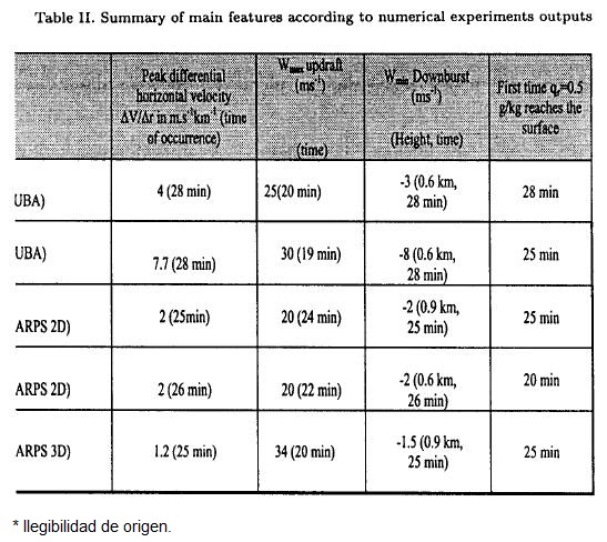
The model version used in the experiment E₂ is the same as in E₃, but a constant value of K_m equal to 160 m² s^-1 is specified in the turbulence treatment. This value has been previously used in a verification test for a deep convective real case (Nicolini, 1993). The temporal evolution of the integration domain peak values and the behavior of the different thermodynamic and dynamic variables in this experiment are similar to those described in the previous one. There is a small temporal lag of about 2 min in the three cloud stages compared to E₃. The horizontal cloud extension (not shown) is around 1 km narrower in the E₂ run, consistent with previous findings where a constant Km version of the same model was used (Nicolini and Paegle, 1989; Nicolini, 1993). Also, both vertical velocities and outflow strength are weaker in E₂, compared to experiment E₃ (see Table II).

A similar sensitivity test to turbulence parameterization has been carried out with the ARPS model in its 2-D version.

The cloud evolution simulated by experiment E₅ is quite similar to E₃, but it lags and produces a weaker convection. This difference may be explained by the inclusion of second and fourth order computational mixing schemes activated in ARPS. The K_m pattern resembles the one corresponding to the UBA model, but is less variable in space (compare Figures 5a and 5b). As there is a coincidence in the Km maximum value attained by both models, in a preliminary test the ARPS was run with the same constant value specified in run E₂ (160 m² s^-1). As this last run (not shown) leads to a shallow and extremely weak convection unable to produce ice and precipitation, a new set of experiments were conducted decreasing the constant turbulent diffusiveness from 160 down to 40 m² s^-1 until an intensity at least as strong as the one obtained in run E₅ is reproduced. The comparable strength in the Experiment E₄, characterized by a K_m value of 40 m² s^-1 compared to E₅ is evident as indicated in Table II, as well as a tendency to a time lag similar to that observed in the UBA model.

An additional experiment (not shown) that incorporates the option of an unsteady 1.5 turbulent kinetic energy closure performed with an ARPS 2-D version leads again to a much weaker convection than in the Smagorinsky-Lilly parameterization case. This set of experiments emphasizes the sensitivity of the 2-D version of ARPS to the whole available turbulence treatments. On the contrary, when the upgraded 1.5 turbulence parameterization is used in the 3-D ARPS version and therefore experiment E₆ is run, the resulting convection seems more reasonable and the updraft strength is more similar to the one reproduced in run E₃. This result might indicate a more reliable performance of this parameterization in a 3-D context. Despite this improvement, the downdraft and the outflow are still weaker compared to E₃. The K_m pattern is more organized and the values more than duplicate those obtained in 2-D experiments (Fig. 5c).

 

5. Concluding remarks

This investigation tested the sensitivity of a bidimensional cloud model with an upgraded turbulence parameterization. This model has the ability to simulate a credible convective scenario in a real data case characterized by observed strong outflows. The main improvements focus on the turbulence parameterization for both model versions (only liquid and mixed phase microphysics respectively) using a first order turbulence closure. In a previous paper (Nicolini and Torres Brizuela, 1999) the formulation of the turbulence scheme is derived, whereas the current paper focuses in exploring model sensitivity. Four experiments were performed to accomplish this objective.

Results show that the new turbulence parameterization affects the simulation of convection. The emphasis is in the representation of one of the significant features of the convective event used for this sensitivity test. Maximum surface wind speed corresponding to the strongest downdraft is better approached by the variable K_m representation. The apparent superior representation of a peak differential horizontal velocity in the Alabama case (Nicolini, 1993) by the previous km constant version of the UBA model might be explained by the fact that a weak horizontal convergence has been imposed for that case consistent with a mesoscale observed convergence. No attempt has been made in the present case to use any initiation technique additional to bubble perturbation to account for the dynamical effect of the cold front. This lack of forcing might lead to weaker simulated winds than those observed (18 ms^-1 instead of 24 ms-1).

Previous results show that both models are sensitive to the turbulence treatment with a stronger impact in the ARPS. Then, the sensitivity of the UBA model to the turbulence parameterization is not one of its peculiar characteristic, although weaker. This difference in sensitivity is difficult to justify given the different architecture (mainly different computational mixing schemes and time filter) of each model. The inclusion of the third dimension in experiment E₆, compared with the 2-D experiments, enhances the vertical motions but reduces the divergent outflows at the surface. Performance of the UBA model proves better than the ARPS 2-D version in terms of convective outflow strength near the surface for this simulated case. This result is encouraging and justifies future validation of the UBA model in other downburst cases in order to asses its capability as a forecast tool in airport activities. Observational data representative of convection over Argentina are needed to gain further understanding on both the environmental conditions and on convection-related phenomena over this region, and for model initialization and validation.

The UBA model dimensional constraint clearly precludes the simulation of 3-D dynamics like rotational features. In turn, it has the advantage of allowing less central computational time (approximately 7 min of CPU in a PC-Pentium II-233MHz).

The Resistencia storm is a warm-cloud-based and weak-shear case similar to the Alabama case documented by Wakimoto and Bringi (1988). They show that in the Alabama storm the microphysical structure of the simulated event is crucial to the microburst generation. Therefore, in this case and despite the fact that for computational economy it is more convenient to use the simplest bulk water microphysics formulation, a more advanced parameterization like the one developed by Carrió and Nicolini (2000) is currently being tested in order to address potential benefits. Attention is focused on a more accurate simulation of the descent of the graupel/hail specie nearer the ground during the dissipation stage.

 

Acknowledgements

This research was supported by CONICET grant PIP N4520/96, ANPCyT grant PICT No 07-00000-01757 and the University of Buenos Aires, grant TX30. The authors wish to thank the Argentina National Weather Service for providing the Resistencia sounding data. Dr. Marcela Torres Brizuela wishes to thank the F. O. M. E. C. for her doctorate fellowship.

 

REFERENCES

Arakawa, A., 1966. Computational design for long term numerical integrations of the equations of atmospheric motion. J. Comp. Phys., 1, 119-143.         [ Links ]

Carrió, G. G. and M. Nicolini, 1999. A double moment warm rain scheme. Description and test within a kinematic framework,. Atmospheric Research, 52, 1-16.         [ Links ]

Carrió, G. G. and M. Nicolini, 2000. A predominant mass preserving scheme for the microphysics of convective clouds. Proceedings, 13th Intern. Conf. On Clouds and Precipitation. Reno, Nevada USA, 14-18 August 2000, 514-517.         [ Links ]

Clark, T. L., 1979. Numerical simulations with a three-dimensional cloud model: Lateral boundary condition experiments and multicellular severe storm simulations. J. Atmos. Sci., 36, 2191-2215.         [ Links ]

Cotton, W. R., and R. A. Anthes, 1989. Storm and Cloud Dynamics. Academic Press, 881 pp.         [ Links ]

Durran, D. R., and J. B. Klemp, 1982. On the effects of moisture on the Brunt-Väisälä frequency. J. Atmos. Sci., 39, 2152-2158.         [ Links ]

Emanuel, K. A., 1986. Overview and definition of mesoscale meteorology. Mesoscale Meteorology and Forecasting, P. S. Ray, American Meteor. Soc., 1-17.         [ Links ]

Emanuel, K. A., 1994. Atmospheric convection. Oxford Univ. Press, New York, 580 pp.         [ Links ]

Klemp, J. B., and R. B. Wilhelmson, 1978. The simulation of three dimensional convective storm dynamics. J. Atmos. Sci., 35, 1070-1096.         [ Links ]

Krueger, S. K., 1988. Numerical simulation of tropical cumulus clouds and their interaction with the subcloud layer. J. Atmos. Sci., 45, 2221-2250.         [ Links ]

Lin, Y. -L, R. D. Farley, and H. D. Orville, 1983. Bulk parameterization of the snow field in a cloud model. J. Climate Appl. Meteor., 22, 1065-1092.         [ Links ]

Lilly, D. K., 1967. The representation of a small-scale turbulence in numerical simulation experiments. Proc. IBM Scientific Computing Symposium on Environmental Sciences. Thomas J. Watson Research Center, Yorktown Heights, N.Y, 195-210.         [ Links ]

Lipps, F. B., and R. S. Hemler, 1982. A scale analysis of deep moist convection and some related numerical calculations. J. Atmos. Sci., 39, 2192-2210.         [ Links ]

Lord, S. J., H. E. Willoughby, and J. M. Pietrowicz, 1984. Role of a parameterized ice-phase microphysics in an axisymmetric, nonhydrostatic tropical cyclone model. J. Atmos. Sci., 41, 2836-2848.         [ Links ]

Mellor, G. L., and T. Yamada, 1974. A hierarchy of turbulence closure models for planetary boundary layers. J. Atmos. Sci., 31, 1791-1806.         [ Links ]

Malkus, J. S., and G. Witt, 1959. The evolution of a convective element: A numerical calculation. The atmosphere and the sea in motion. Rockefeller Institute Press, New York, 425-439.         [ Links ]

Nicolini, M., 1986. Interacción dinámica del entorno con la convección en nubes cumulus [Dynamical interaction of the environment with convection in cumulus clouds]. Doctoral dissertation, University of Buenos Aires, Argentina, 317 pp. [Available from the author at Depto. de Ciencias de la Atmósfera y los Océanos, Univ. de Buenos Aires, Pab. II, Ciudad Universitaria, 1428 Buenos Aires, Argentina]         [ Links ].

Nicolini, M., 1993. Simulación numérica de una tormenta generadora de una "microburst", su verificación. [Numerical simulation of a microburst producing storm, its verification]. Meteorológica, 18, 23-32.         [ Links ]

Nicolini, M., and J. Paegle, 1989. Real data deterministic forecasts of ambient vertical motion fields upon convective precipitation. Second Int. Cloud Modelling Workshop/Conf., Toulouse, France. WMO/TD-No 268, 207-220.         [ Links ]

Nicolini, M., K. M. Walton and J. Paegle, 1993. Diurnal oscillations of low-level jets, vertical motion, and precipitation. A model case study. Mon. Wea. Rev., 121, 9, 2588-2609.         [ Links ]

Nicolini, M., and M. Torres Brizuela, 1997. Estadística de vientos fuertes asociados a convección en Ezeiza y Resistencia y estudio numérico de los forzantes en un caso real [Convective strong winds statistics at Ezeiza and Resistencia and a numerical study of forcings in a real case] Meteorológica, 22, 19-35.         [ Links ]

Nicolini, M., and M. Torres Brizuela, 1999. A description of the University of Buenos Aires two-dimensional deep convective model: theoretical background of an upgraded turbulence parameterization. Meteorológica, 24, 23-34.         [ Links ]

Orlanski, I., 1975. A rational subdivision of scales for atmospheric processes. Bull. Amer. Meteor. Soc., 55, 527-530.         [ Links ]

Proctor, F. H., 1989. Numerical Simulations of an isolated microburst. Part II: Sensitivity experiments. J. Atmos. Sci., 46, 2143-2165.         [ Links ]

Smolarkiewicz, P. K., and T. L. Clark, 1986. The multidimensional positive definite advection transport algorithm. Further development and applications. J. Comp. Phys., 67, 2, 394-438.         [ Links ]

Tag, P. M., F. W. Murray, and L. Randall Koening, 1979. A Comparison of several forms of eddy viscosity parameterization in a two-dimensional cloud model. J. of Applied Meteorology, 18, 1429-1441.         [ Links ]

Tuttle, J. D., V. N. Bringi, H .D. Orville and F. J. Kopp, 1989. Multiparameter radar study of a microburst: Comparison with model results. J. Atmos. Sci., 46, 601-620.         [ Links ]

Uliasz, M., 1994. Subgrid scale parameterizations. Mesoscale modeling of the atmosphere. R. A. Pielke and R. Pearce, Ed., American Meteorological Society, 13-19.         [ Links ]

Wakimoto, R. M. and V. N. Bringi, 1988. Dual-polarization observations of microbursts associated with intense convection: The 20 July storm during the MIST Project. Mon. Wca. Rev., 116, 1521-1538.         [ Links ]

Xue, M., K. Droegemeier and V. Wong, 1995. The advanced regional prediction system and real-time storm weather prediction. Proceedings of the Internat. Workshop on limited-area and variable resolution models, Beijing, China, World Meteorological Org.         [ Links ]