On the stability of atmospheric waves with low wave numbers

 

A. Wiin-Nielsen

The Collstrup Foundation, The Royal Danish Academy of Sciences and Letters H.C. Andersens Blvd. 87, DK-155S Copenhagen V, Denmark

 

(Manuscript received Feb. 21, 2000; accepted in final form May 17, 2000)

 

RESUMEN

Se investiga la estabilidad de las ondas atmosféricas con número bajo de ondas, mediante un modelo quasi-geostrófico de segunda clase. Tal modelo está basado en la ecuación termodinámica, la de continuidad y un empleo riguroso de las relaciones geostróficas.

La condición de frontera en la superficie terrestre se formula de dos maneras. Los efectos de una condición fronteriza a los 1000 hPa, donde la velocidad vertical P es nula, se compara con los efectos de una segunda condición, donde W es cero. Las dos condiciones fronterizas se usan para determinar la estabilidad de las ondas de número bajo.

La segunda condición introduce ondas grandes, tanto con velocidades de fase positivas como negativas, especialmente en las bajas latitudes, pero tiene también una influencia sobre la estabilidad de estas ondas.

El resultado principal de la investigación comparativa es que entre más realista es la condición de frontera, en general producirá inestabilidades mayores que la condición de frontera más simple.

Los tiempos de pliegue en e, obtenidos con el modelo más general concuerdan mejor con los resultados obtenidos mediante las observaciones.

 

ABSTRACT

The stability of atmospheric waves with low wave numbers is investigated using a quasi-geostrophic model of the second kind. Such a model is based on the thermodynamic equation, the continuity equation and a rigorous use of the geostrophic relations.

The boundary condition at the surface of the Earth is formulated in two ways. The effects of a boundary condition at 1000 hpa, where the vertical p-velocity is zero, is compared with the effects of a second condition, where w is zero. The two boundary conditions are used to determine the stability of the low wave number waves.

The second condition introduces waves with large positive and negative phase velocities, especially in the low latitudes, but has also an influence on the stability of these waves.

The main result of the comparative investigation is that the more correct boundary condition in general will produce stronger instabilities than the simpler boundary condition. The e-folding times obtained with the more general model is in closer agreement with the results obtained by observational studies.

 

1. Introduction

The transient atmospheric waves with low wave numbers have been investigated in various ways and for various reasons since hemispheric and global analyses of the state of the atmosphere became possible. Some of these studies have been concerned with the amplitude and wave speed of the observed transient waves (Deland, 1964, Deland and Lin, 1967, Eliasen and Machenhauer, 1965 and 1969, Bradley and Wiin-Nielsen, 1968). Other investigations have focused on periodicities connected with the low wave number waves such as a 5-day periodicity (Madden and Julian, 1972, Geisler and Dickenson 1976), while still other studies have been made of the low wave number waves in the stratosphere (Hirota and Hirooka, 1984 and references in their paper) and of the normal modes of the low wave number waves (Salby, 1981, a and b).

Early studies of the dynamcs of low wave number waves in simple baroclinic models were carried out by Wiin-Nielsen (1961, a and b), Miles (1965), Bradley and Wiin-Nielsen (1968), Wiin-Nielsen (1971) and Fisher and Wiin-Nielsen (1971). Kasahara (1976) has considered the effect of the zonal flows on the free oscillatons in a barotropic atmosphere.

The atmosphere contains waves on many scales. The creation of waves on the middle scale is described as a result of barotropic and baroclinic instabilities. The transient atmospheric waves with small wave numbers are more difficult to describe using the standard quasi-geostrophic models, partly because instabilities of the right order of magnitude are difficult to obtain, and partly because the speed of the waves in the model is dominated by the beta-effect.

The atmospheric energy spectra in wave number space based on observations contain considerable energy in the low wave numbers (Wiin-Nielsen, 1967). These waves have both a stationary and a transient part of which the stationary part to some extent is produced by a topographical forcing (Charney and Eliassen, 1949) and from the forcing due to the stationary heat sources and sinks (Smagorinsky, 1953). We shall be concerned with the transient part of these waves. The spectra of atmospheric energies show in general that the small wave numbers contain considerable amounts of both available potential and kinetic energy In spectra calculated from observations for winter months in the Northern Hemisphere the amount of energy in the low wave numbers may occasionally be very large. The spectra of energy conversions indicate for low wave numbers that the transient part may give a considerable contribution to the total energy conversion (Wiin-Nielsen and Chen, 1993, Chapter 9).

Investigations of the nonlinear exchange of energy among waves (Saltzman and Teweles, 1964, Yang, 1967, Chen and Wiin-Nielsen, 1978) show that the eddy available energy is cascaded from the smaller to the larger wave numbers, while kinetic energy is cascaded from wave numbers of a medium size towards both the small and the large wave numbers. However, the amounts of kinetic energy cascaded to the low wavenumbers is on average very small (about 0.1 W m^–2), and it is doubtful if this process alone can account for the relatively large amount of kinetic energy in the low wave number transient waves. The low wave number waves will loose more available potential energy to the higher wave numbers than the kinetic energy received from the same waves.

The transient waves with low wave numbers may also be influenced by the topography and the heat sources and sinks. We have thus three physical processes that may influence the creation and the behavior of the waves with small wave numbers. The purpose of the paper is to concentrate on possible instabilities of the low wave number waves in order to account for the phase speed and possible instabilities for these waves. It may thus be of interest to examine the baroclinic stability of the waves with low wave numbers.

Stability investigations of atmospheric waves are mostly based on the quasi-geostrophic equations. The general quasi-geostrophic atmospheric models are valid for wave numbers of moderate size. For example, a perturbation analysis of a two level, quasi-geostrophic model indicates that the speed of low wave number waves should be from east to west with considerable magnitudes and comparable to the Rossby speeds: U — β/k². These models are therefore quite unrealistic for the low wave numbers. For waves with small wave numbers the model should employ spherical geometry. In addition, scale analysis shows that for these waves the ordinary quasi-geostrophic model equations should be replaced by a different set of equations (Philips, 1963). As a first approximation a strict use of the geostrophic relation can be applied. A model for the low wave number waves may thus be based on the geostrophic relations, the thermodynamic equaton, the continuity equation and the proper boundary conditions at the top of the atmosphere and at the surface of the Earth. Such a model is called a quasi-geostrophic model of the second kind by Phillips (loc. cit.). It should be emphasized that the described model may only be a first approximation to a description of the transient low wave number waves, because the scale analysis does not involve the meridional scales. Without forcing and dissipation the model conserves potential energy. Burger (1958) was the first to emphasize the special conditions applicable to the low wave number waves. He showed also that Charney's model (1947) was unstable almost everywhere. Burger has returned to the problem in later publications (Burger, 1988 and 1991).

The possible instability of the low wave number waves was investigated in a preliminary way by Welander (1961) and Wiin-Nielsen (1961a, 1961b), but an expanded investigation was carried out by Fisher and Wiin-Nielsen (1971). The latter investigation applied very simple assumptions, because a single analytical solution of the stability problem was required for computational reasons. Assuming that the vertical variation of the basic zonal wind is linear, and that the basic state static stability parameter varies as p^–1, but disregarding any meridional variation of these two parameters in the basic state, it was possible to obtain analytical solutions expressed in hyper-geometrical functions, and numerical solutions were then produced using the so-called shooting method.

Lynch (1979) has emphasized the lower boundary condition for the low wave number waves and has formulated this boundary condition in terms of the geopotential. His treatment of the lower boundary condition includes the advection term of pressure on a surface where the geopotential is constant or the advection of the geopotential on a constant pressure surface, but since the model applies geostrophic conditions in a strict sense, the advection term vanishes.

The purposes of the present investigation is to expand the stability studies of the low wave number waves and to compare the solutions of the stability problem using two different lower boundary conditions. In one of them it is assumed that the vertical p-velocity (ω) vanishes at the lower boundary, while in the other it is assumed that w = 0 at the surface of the Earth. The latter condition is expressed as a differential equation in the vertical p-velocity.

We shall first investigate the very simple case of a constant basic zonal wind and a constant value of the stability parameter. Although this case is unrealistic, it can serve to illustrate the effect of a non-zero lower boundary condition on the speed of the wave and the stability. The next cases will be a determination of the stability of the very long waves using more realistic basic states obtained from observations or from simpler basic baroclinic states. The zonal state of wind and temperature, averaged for January 1999, is the starting point. From the zonally averaged, observed temperature field the static stability parameter was computed as a function of latitude and pressure. From the observed and computed fields we use the data at 0, 250, 500, 750 and 1000 hPa for the zonal winds, while the stability parameter is needed at 250, 500 and 750 hPa.

A comparison is made between

(a) the results for a full variation of the static stability parameter and the zonal wind in the basic state, and

(b) a case, where these parameters vary with pressure only.

 

2. The basic equations and the boundary conditions

The equation for the stability problem has been derived in detail by Fisher and Wiin-Nielsen (1971) in a form where the perturbation vertical p-velocity is the dependent variable. This equation is given in (2.1).

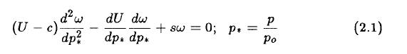
U and c have the dimension of m per s. In addition, the independent variable is p_* = p/p₀, where p₀ is equal to 1000 hPa. The static stability parameter, s, is given in (2.2).

The subscript z indicates a zonal average.

The variation of s with latitude is due to the Coriolis parameter and to the specified static stability in the basic state. (2.1) cannot be applied at the equator. The latitude interval which will be used is from 15 to 85 degrees north. The variation of the trigonometric part of s is shown in Figure 1. Large values are obtained at the low latitudes and the quantity vanishes at the North Pole. It is emphasized that latitude enters only as a parameter, and each latitude can be treated independent of the other latitudes in the stability analysis applying, however, the proper zonal winds and static stabilities. At each latitude we need to know the zonal wind and the static stability parameter in the basic state as functions of pressure. This property of the perturbation equation for the quasi-geostrophic motion of the second kind is a peculiar fact that is a result of the scale analysis for low wave number waves, where the vorticity equation reduces to the geostrophic relation. However, this nature of the problem does not mean that the resulting perturbations are uncoupled with respect to latitude. The geopotentials and temperatures which may be computed from the solution should be obtained by an integration with respect to latitude, and these parameters will thus connect the various latitudes.

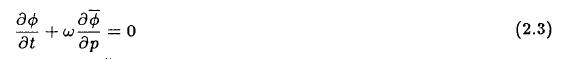
The upper boundary condition will in all cases be ω = 0, while the lower boundary condition will be either w = 0 or w = 0. With good approximation we may write the linearized form of the second version of the boundary condition as given in (2.3).

When we introduce the perturbations and eliminate the geopotential we get the lower boundary expressed in terms of the vertical p-velocity. The final form is given in (2.4) applicable at p_* = 1.

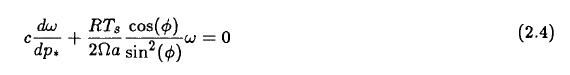
In (2.4) R is the gas constant, T_s a standard value of the surface temperature and Ω the angular velocty of the Earth. This relation, containing only the vertical p-velocity and applied at the 1000 hpa surface, may be added to the equations where the dependent variables are the perturbation vertical p-velocities at the selected levels. The derivative appearing in (2.4) has to be calculated as a non-centered finite difference between the lower boundary and the model pressure level immediately above the 1000 hPa surface, whereby the system of equations will be closed.

It was thus decided to use vertical finite differences, but in this case the eigenvalue problem will not be in the standard form. It was thus decided to use a relatively coarse vertical resolution.

 

3. Simple cases

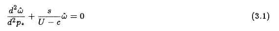
The equations given in section 2 are first applied to the simple case where it is assumed that the zonal wind and the static stability (σ_z) at a given latitude does not vary with pressure. In the case treated below the latitudes were selected to be 15 and 45 deg. north. For this simple case the basic equation (2.1) reduces to the one given in (3.1).

For the case where it is assumed that the vertical p-velocity vanishes at the lower boundary we find a solution which may be written in the form given in (3.2), where n is an integer.

We have thus an infinite number of solutions, but the modes for the larger values of n will be very close to the constant zonal velocity. The other case with the second lower boundary condition is a little more cumbersome. We divide the discussion in two parts and consider first solutions where c < U. In this case the solutions are trigonometric functions. The upper boundary condition requires that the coefficient of the cosine-term is zero. Using next the lower boundary condition, we may write the result of applying the boundary conditions at p_* = 1 in the form given in (3.3).

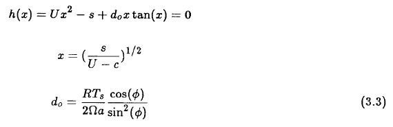
The real roots of H(x) are found by numerical methods whereafter c is determined by the second relation in (3.3).

The second case is c > U. In this case we have exponential solutions. Applying the upper and the lower boundary condition at p_* = 1 we may express the equation for the phase velocity as given in (3.4).

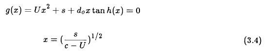
The real zeroes of g(x) are determined by numerical methods.

To illustrate the difference between the two boundary conditions we shall select evaluations at 15 and 45 degrees of latitude. For each case the equations (3.3) and (3.4) were solved for x by numerical procedures, whereafter c was obtained from the equations relating c to x. For the case with c < U it is also possible to find negative values of x, but except for a numerically large value the negative and positive values of x have about the same absolute size. In view of this remark one obtains the same value for the phase velocity since only x² enters in these relations. Negative values of x have therefore not been included in the calculations. The results may be seen in Table 1, where the values computed with the simple lower boundary condition (ω = 0) are compared with the values obtained from the more realistic differential boundary condition.

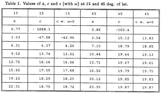
The main difference between the results from the two boundary conditions for the two selected latitudes is that the differential condition introduces a fast moving wawe with large negative values. The other wave speeds are comparable in size, and both sets will for the higher modes approach the adopted value of U = 20 m per s. It is also seen that the difference between the phase velocities for the higher modes are almost the same. It is apparent from the table that the wave with the large wave speed is very large at the low latitude of 15 degrees.

Although we have included only the latitudes 15 and 45 degrees in the table, similar results are obtained for all the other latitudes.

We consider next the case where c > U corresponding to solutions with exponential functions, see (3.4). With the chosen numerical values of U = 20 m per s and ω = 4x10^–6 m⁴ s² kg^–2 and T_s = 288 K we find no real solutions to the equation. Figure 2 shows the function g(x) defined in (3.4), and it is seen that the curve does not reach the x–axis. This result does not depend critically on the chosen value of the static stability. It is seen from the analysis of the above simple case that a main effect of the second boundary condition is to introduce fast moving waves with unrealistic large velocities.

The next example will illustrate the effect of the vertical wind shear. In this second simple case we disregard the static stability factor whereafter the basic perturbation reduces to the equation in (3.5).

(3.5) can be solved directly. After the application of the upper boundary condition we may write the solution in the form given in (3.6).

Application of the simple lower boundary condition of a vanishing vertical p-velocity gives the result in equation (3.7).

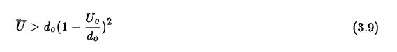
while the second lower boundary condition leads to the equation (3.8) for the phase velocity, c.

Instability will thus be present if the vertical mean velocity satisfies the inequality shown in (3.9).

The critical value of the vertical mean velocity is shown in Figure 3. It is seen that for a given value of the vertical mean velocity instability will be present in the higher latitudes. For example a vertical mean value will as shown on the figure give instability north of about 50 degrees of latitude. Figure 4 shows the real solutions as a function of latitude, while Figure 5 gives the e-folding time in days for the unstable cases. It is seen that rather small values of the e-folding time are found in the high latitudes. We may thus conclude from the simple cases that, taken in isolation, the static stability is a stabilizing effect, while the vertical wind shear is a destabilizing effect which results in instability in the high latitudes where the stabilizing effect from the lower boundary condition is small.

 

4. The more general cases

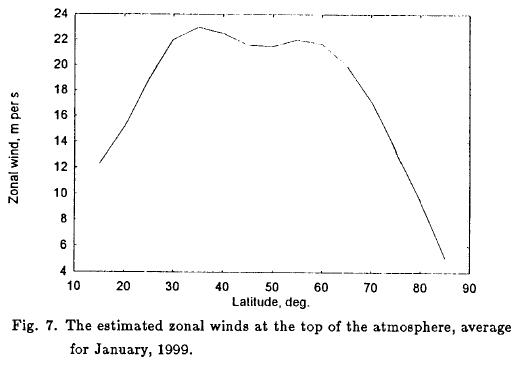
We return to the basic equation for the model for the low wave numbers. We shall restrict the considerations to a limited vertical resolution by selecting the levels at the pressure surfaces 0, 250, 500, 750 and 1000 hPa. As a basic, stationary state it was decided to use data averaged for the month of January, 1999, for which the zonally averaged winds and temperatures are available. The zonally averaged winds for the four surfaces 250, 500, 750 and 1000 hPa are shown in Figure 6 from 15 to 85 degrees of latitude, while the estimated zonal wind at the top of the atmosphere is shown in Figure 7. All the wind data were obtained either directly or by interpolation using the winds at pressure surfaces above and below the level in question. The winds and temperatures are available at 31 vertical levels.

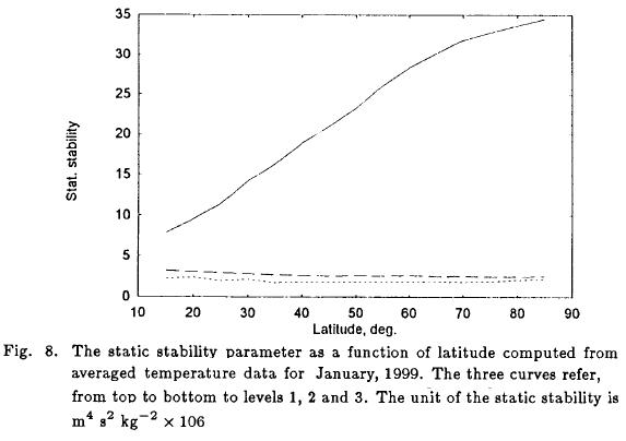
The static stability (σ_z) was calculated from the temperature data. The variation with latitude of the static stability at the levels 250, 500 and 750 hPa are shown in Figure 8. The static stability is relatively small and the dependence on latitude is also small at the levels 500 and 750 hPa, while the variation at 250 hPa is large ranging from small values in the low latitudes to large values at high latitudes.

In the five level model we need winds at all five levels, while the static stability parameter is needed only at the levels 250, 500 and 750 hPa. With the boundary condition of w = 0 at p = 0 used in all calculations the finite difference equations for the levels 250, 500 and 750 hPa were obtained giving three equations. In the case where we apply a non-zero vertical velocity at the 1000 hPa, the boundary condition will give one additional equation. For the general case we have thus a 4 x 4 matrix for the determination of the eigen-values, while we have a 3 X 3 matrix for the boundary condition where ω = 0 at 1000 hPa.

The determinant was evaluated in the two cases resulting in a fourth and a third degree equation with real coefficients and with the eigenvalue, c, as the unknown in the two cases. These two equations were solved by numerical methods giving both real and complex roots.

Figure 9 shows the e-folding times for the two cases. In the numerical solutions it was decided to use the value zero for the stable cases, since it is impossible to plot a value of infinity. The dashed curve indicates instability from 25 to 65 degrees of latitude and also a weak instability at 75 degrees of latitude. The e-folding times are generally large with values varying from 14 to more than 30 days. The solid curve obtained using the non-zero boundary condition at 1000 hPa indicates e-folding times which are much smaller from 25 to 60 degrees of latitude with values of only a few days. This result is in general agreement with the results obtained from observational studies by Haurwitz (1937) who finds e-folding times for the long waves of the same order of magnitude.

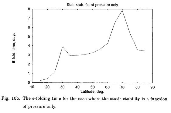
It is of interest to investigate the importance of the meridional variation of the static stability. The real variation of the static stability parameter was therefore replaced by a variation with pressure only where the values at a given pressure level are taken as the meridional average.

Using first the boundary condition of a vanishing vertical p-velocity at 1000 hPa the results displayed in Figure 10a are found, where the curve shows the e-folding time with a full variation of the static stability parameter. Figure 10b shows the curve obtained when the static stability parameter is a function of pressure only. The simple variation gives shorter e-folding times in the low latitudes, while minor differences appear at the other latitudes.

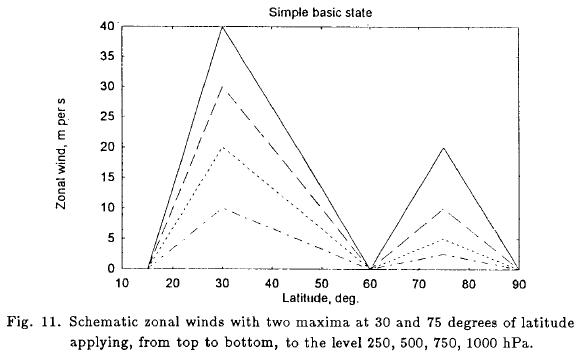
The use of the observed averaged state for January 1999 as a basic steady state for the zonally averaged wind and static stability is not necessary to obtain the demonstrated instabilities. This basic state was replaced by schematic zonal winds as shown in Figure 11. This wind distribution simulates in a very simple and schematic way a zonal state with a subtropical and a polar jet. The static stability was replaced by constant values for the 500 and 750 hPa surfaces. At 250 hPa the static stability varied linearly from a value of 5 X 10^-6 m⁴ s² kg^-2 at 15 degrees of latitude to 35 x 10^-6 m⁴ s² kg^-2 at the North Pole. The resulting e-folding times for the two boundary conditions are seen in Figure 12. The dashed curve applies to the vanishing p-velocity at the surface. Neutrality is present except at 65 degrees where a weak instability is found. The solid curve indicates the e-folding times for the second lower boundary condition. Instabilities with e-folding times of 2 to 5 days are found from 25 degrees to 50 degrees of latitude, and a very weak instability is also found at 65 degrees of latitude in this case.

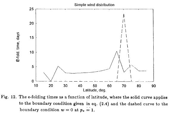
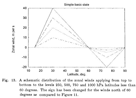
When we replace the polar westerly jet with an easterly jet of the same strength as shown in Figure 13 and repeat the stability investigation we find the results seen in Figure 14. The case with a vanishing vertical p-velocity at the lower level is stable in this case as seen by the dashed line from 15 to 85 degrees on the abscissa, while the non-zero boundary condition gives instability from 25 to 50 degrees of latitude and weak instabilities from 60 to 85 degrees of latitude.

 

5. Concluding remarks

The use of the quasi-geostrophic model of the second kind on the stability of the low wave number waves has resulted in the determination of instabilities which have the smaller e-folding times in connection with the subtropical zonal wind maximum and very weak instability in the higher latitudes. Two different boundary conditions applied at 1000 hPa have been compared. The general result is that the boundary condition of w = 0, resulting in the approximative formulation given in eq. (2.4), leads to smaller e-folding times than the boundary condition ω = 0 at 1000 hPa.

Another general result is that the non-zero boundary condition introduces two fast moving waves with positive and negative wave speeds that become particularly large in the low latitudes.

These waves are not found in the real atmosphere. The presence of these waves will require the use of small time steps if the basic nonlinear equations for the geostrophic model of the second kind were to be integrated numerically. Results of the described type are obtained for basic states based on observations or described by schematic distributions of the vertical and meridional variations of the zonal winds and the static stability.

The analyses used in the present paper are based on the equations of a geostrophic model of the second kind as described by Phillips (1963). The formulation of the basic equations is based on a scale analysis for low wave number waves. It would appear, both from the remarks by Phillips (loc.cit.) and from the results in this paper that the applied equations may be too simplified. It may be an advantage to use a vorticity equation in which the local time derivative is neglected, while the vorticity advection is maintained as was done by Wiin-Nielsen (1961a) although the model was restricted to a two-level model on the beta-plane. It is hoped that the present investigation will be expanded to such a model maintaining the spherical geometry and a proper lower boundary condition.

 

REFERENCES

Bradley, J. H. S. and A. Wiin-Nielsen, 1968. On the transient part of the atmospheric planetary waves, Tellus, 20, 533-544.         [ Links ]

Burger, A. P., 1958. Scale considerations of planetary motions of the atmosphere, Tellus, 10, 195-205.         [ Links ]

Burger, A. P., 1988. Static stability and vertical velocity: from planetary to small scale, Tellus, 40A, 353-357.         [ Links ]

Burger, A. P., 1991. The potential vorticity equation: from planetary to small scale, Tellus, 43A, 191-197.         [ Links ]

Charney, J. G. and A. Eliassen, 1949. A numerical method for predicting the perturbations in the middle latitudes, Tellus, 1, 38-54.         [ Links ]

Chen, T.-C. and A. Wiin-Nielsen, 1978. On nonlinear cascades of atmospheric energy and enstrophy in a two-dimensional index, Tellus, 30, 313-332.         [ Links ]

Deland, R. J., 1964. Travelling planetary waves, Tellus, 16, 271-273.         [ Links ]

Deland, R. J. and Y. -J. Lin, 1967. On the movement and prediction of travelling planetary waves, Mo. Wea. Rev., 95, 21-31.         [ Links ]

Eliasen, E. and B. Machenhauer, 1965. A study of the fluctuations of the atmospheric, planetary flow pattern represented by spherical harmonics, Tellus, 17, 220-238.         [ Links ]

Eliasen, E. and B. Machenhauer, 1969. On the observed large-scale atmospheric wave motion, Tellus, 21, 149-166.         [ Links ]

Fisher, P. W. and A. Wiin-Nielsen, 1971. On baroclinic instability of ultra-long waves, Tellus, 23, 269-284.         [ Links ]

Geisler, J. E. and R. E. Dickenson, 1976. The five-day wave on the sphere with realistic zonal winds, Jour. Atmos. Sci., 33, 632-641.         [ Links ]

Haurwitz, B., 1937. The oscillations of the atmosphere, Beitr. Geophys., 51, 195-233.         [ Links ]

Hirota, I. and T. Hirooka, 1984. Normal mode Rossby waves observed in the upper stratosphere, Part I: First symmetric modes of zonal wave number 1 and 2, Jour. Atmos. Sci., 41, 1, 1253–1267.         [ Links ]

Kasahara, A., 1976. Normal modes of ultra-long waves in the atmosphere, Mo. Wea. Rev., 104, 669-690.         [ Links ]

Lynch, P., 1979, Baroclinic instability of ultra-long waves modelled by planetary geostrophic equations, Geophys. Astrophys. Fluid Dynamics, 13, 107-124.         [ Links ]

Madden, R. A. and P. Julian, 1972. Further evidence of global-scale 5-day pressure waves, Jour. Atmos. Sci., 29, 1464-1469.         [ Links ]

Miles, J. W., 1965. Instability of very long waves in a zonal flow, Tellus, 17, 302-305.         [ Links ]

Phillips, N. A., 1963. Geostrophic motion, Rev. of Geophysics, Vol. 1 No. 2, 123-176.         [ Links ]

Salby, M. L., 1981a. Rossby normal modes in non-uniform background configuration, Part I, Jour. Atmos. Sci., 38, 1803-1826.         [ Links ]

Salby, M. L., 1981b. Rossby normal modes in non-uniform background configuration, Part II, Jour. Atmos. Sci., 38, 1827-1840.         [ Links ]

Saltzman, B. and S. Teweles, 1964. Further statistics on the exchange of kinetic energy between harmonic components of the atmospheric flow, Tellus, 16, 432-35.         [ Links ]

Smagorinsky, J., 1953. The dynamical influence of large-scale heat sources and sinks on the quasi-stationary mean motions in the atmosphere, Quart. J. Roy. Met. Soc., 79, 342-366.         [ Links ]

Welander, P., 1961. Theory of very long waves in a zonal atmospheric flow, Tellus, 13, 140-155.         [ Links ]

Wiin-Nielsen, A., 1961a. A preliminary study of the dynamics of transient, planetary waves in the atmosphere, Tellus, 13, 320-333.         [ Links ]

Wiin-Nielsen, A. 1961b. A note on the behavior of very long waves in simple baroclinic models, Jour, of Meteor., 18, No. 2, 204-207.         [ Links ]

Wiin-Nielsen, A., 1967. On the annual variation and spectral distribution of atmospheric energy, Tellus, 19, 540-559.         [ Links ]

Wiin-Nielsen, A., 1971. On the motion of various vertical modes of the transient very long waves, Part II: the spherical case, Tellus, 23, 207-217.         [ Links ]

Wiin-Nielsen, A. and T. -C. Chen, 1993. Fundamentals of atmospheric energetics, Oxford University Press, 376 pp.         [ Links ]

Yang, C.-H., 1967. Nonlinear aspects of the large-scale motion in the atmosphere, Univ. of Michigan, Sci. Report: 08759-1-T, 173 pp.         [ Links ]