A note on the logarithmic -3 law of atmospheric energy

 

A. WIIN-NIELSEN

Geophysical Department, Niels Bohr Institute for Astronomy, Physics and Geophysics Juliane Maries Vej 30 DK-2100 Copenhagen, Denmark.

 

(Manuscript received May 11, 1999; accepted in final form Aug. 17, 1999)

 

RESUMEN

Las observaciones muestran que la energía cinética atmosférica, en promedio, obedece a una relación que dice que su dependencia del número de onda longitudinal es n⁻³, en un intervalo con números de onda mayores que el de conversión máxima, desde la energía potencial torbellinaria disponible hacia la propia energía cinética y los números de onda denominados por la disipación debida al rozamiento. Los experimentos numéricos con un modelo barotrópico han demostrado que la ley exponencial para la energía cinética es n⁻¹ en los números de onda pequeños. Tales relaciones resultan del forzamiento que tiene su origen en el calentamiento diabático; los procesos de energía cinética en cascada, asociados a las interacciones no lineales, y la disipación por rozamiento.

El trabajo presenta el estudio de un fluido homogéneo con una superficie libre forzada por adición y sustración de fluido. Para un forzamiento dado, el estado de permanencia puede determinarse, aunque el modelo no sea lineal. Para un forzamiento especial, el espectro de energía cinética muestra exponentes de −1 y −3. Una cuestión importante es si la energía potencial también obedece a una ley exponencial de exponente igual a −3. Se investigan otros casos de forzamiento a fin de determinar la sensibilidad de los resultados al forzamiento.

 

ABSTRACT

Observations show that the atmospheric kinetic energy on average obeys a relation saying that its dependence on the longitudinal wave number is n⁻³ in an interval with wave numbers larger than the wave number with maximal conversion of eddy available potential energy to eddy kinetic energy and the wave numbers dominated by frictional dissipation. Numerical experiments with a barotropic model have indicated that the power law for the kinetic energy is n⁻¹ for the small wave numbers. Such relations are a result of the atmospheric forcing due to the diabatic heating, the cascade processes of kinetic energy due to nonlinear interactions and the frictional dissipation.

The paper presents a study of a homogeneous fluid with a free surface forced by adding and subtracting fluid. For a given forcing the steady state may be determined although the model is nonlinear. For a special forcing the kinetic energy spectrum shows the −1 and the −3 relations. An important question is whether the potential energy also obeys a −3 power law. Other cases of the forcing are investigated in order to determine the sensitivity of the results to the forcing.

 

1. Introduction

The first paper on the spectral distribution of atmospheric kinetic energy was produced by Fjørtoft (1953). He pointed out, based on the conservation of kinetic energy and enstrophy for a barotropic fluid, that energy added to the atmospheric motion at a certain scale will result in energy cascades influencing both the smaller and the larger wave numbers. A study of the spectral distribution of the kinetic energy based on observations was carried out by Horn and Bryson (1963). They found that the spectral distribution of the kinetic energy for the larger wave numbers could be approximated by a distribution proportional to n^−8/3. A similar result, but with a somewhat different coefficient, was found by Wiin-Nielsen (1967) who found that the best approximation to the data was n^−8/3. A study by Charney (1971) with a continuous vertical variation in a quasi-geostrophic model resulted in a theoretical spectral distribution of the kinetic energy with a variation depending on wave number as n⁻³. Merilees and Warn (1972) pointed out that investigations similar to Charney's study, but based on multilevel models result in distributions with different slopes depending on the number of levels in the model. For example, a two-level quasi-geostrophic model should have a −5 law for the available potential energy and a −3 law for the kinetic energy as found by Steinberg et al. (1971). The −3 law was verified by model integrations carried out by Julian et al. (1970), Kao (1970) and Kao and Wendell (1970) using different general circulation models.

Kraichnan (1967) and Leith (1968 and 1971) made theoretical studies of two-dimensional turbulence and the resulting limited predictability and could also find the −3 law using very simple models based on the advection equation. Lilly (1969) made a numerical simulation using the barotropic vorticity equation in two dimensions with a specified forcing and determined not only the −3 law, but also a −1 law for the small wave numbers. Similar integrations using a two-level, quasi-geostrophic model have been done by Barros and Wiin-Nielsen (1974). Since then the research on the power laws of the energy seems to have stopped. A summary of the research may be found in Wiin-Nielsen and Chen (1993), where it is pointed out that the ideas of inertial subranges may not be valid. However, the two laws were approximated by Wiin-Nielsen (1998) using a numerical integration of a simple model based on the first equation of motion in the spectral domain employing a Newtonian forcing expressed in wave number space.

The purpose of the present paper is to use a model of a homogeneous and incompressible fluid with a free surface and with a forcing consisting of addition and subtraction of fluid (corresponding to the heating of the atmosphere). The basic equations are therefore the first equation of motion in one space dimension and the continuity equation treated in a similar way. The forcing function will be defined as a function of the wave number.

 

2. The model

The model equations will use one space dimension (x) and time (t). The dependent variables will be the velocity component in the x-direction (u) and the geopotential (ɸ). It should be noted that the advection term in the continuity equation gives no contribution since the fluid is assumed to be homogeneous. Equation (2.1) gives the equations.

ɸ₀ is a standard value of the geopotential. They are transformed to wave number space. To make the calculations more convenient we shall define the velocity component as a series in sine-functions giving vanishing velocities at both ends of the interval while the geopotential and the forcing (S) will be defined as series in the cosine-functions giving a vanishing derivative with respect to x at both end of the interval. With these assumptions we may write the spectral equations in the form:

The two sums in the first equation of (2.2) are defined in (2.3)

If we first consider the steady state problem, it is seen from the second equation in (2.2) that the values of u[n] are related to the corresponding term of S[n]. Having the values of u[n] one may determine φ[n] from the first equation. It is then required to calculate the two sums given in (2.3) and the dissipation term. In the non-steady case it will be required to integrate the two equations i (2.2) numerically.

 

3. The experiments

The forcing is specified by the values of S[n]. From the steady state solution it is seen that if the forcing varies as n^p, then u[n] will vary as n^p−1 and u[n]² as n^2(p−1). If we want to generate a wave number variation of n⁻³ for the kinetic energy it will require that p = −1/2, while a kinetic energy varying as n⁻¹ is created by p = 1/2. These results are obtained from the second steady state equation. Similar results for the geopotential cannot be obtained from the first steady state equation due to the nonlinear sums. The main question is therefore if specification of the forcing with a coefficient close to −1/2 which will produce a distribution close to the -3 law for the kinetic energy also will result in a power law close to -3 for the spectral representation of the available potential energy. These considerations result then in a specification of S[n] as given in (2.4).

In (2.4) n_s is the wave number for which the model will have the maximum forcing, S₀. The forcing based on (2.4) is shown in Figure 1 for S₀ = 1, n_s = 7 and p = 1/2. In a more general model such as for example a two-level, quasi-geostrophic model, where the forcing is determined by the heating, the velocity field is forced by the conversion of eddy available potential energy to eddy kinetic energy. This forcing will be at a maximum close to the wave number of maximum baroclinic instability. It is thus reasonable to specify S[n] as similar to the spectral distribution of C(A_E, K_E). Observational studies of the energy conversion C(A_E, K_E) show a maximum at wavenumber n = 7 and falls to smaller values for both smaller and larger wave numbers, when the contribution from the stationary waves are removed (Wiin-Nielsen and Chen, 1993), and the specific shape in Figure 1 depending on n^p and n^−p are thus justified as a possible definition.

The calculations are performed in the following way. From the given values of S[n] we compute u[n] from the second equations. The first equation permits then a numerical determination of φ[n]. For the definition of S[n] given in (2.4) u[n] will for p = 1/2 vary as seen in Figure 2 where the discontinuity for n_s = 7 is seen. Figure 3 shows the distribution of φ[n]with a maximum at n = 12.

Since we are interested in the dependence on n we have in Figure 4 shown the dependence of log (u[n]²/2) on log [n] where the ordinate is the logarithmic contribution from wave number n to the kinetic energy. As expected we find a regime for the small wave numbers where the slope is -1, while the slope for the larger wave numbers is -3. Figure 5 shows a similar arrangement for the potential energy. The minimum in the curve occurs for ln(n) ≈ 2 corresponding to n ≈ 7. At this maximum value of the forcing the eddy potential energy is small due to a large conversion to eddy kinetic energy. For larger values of the wave numbers we obtain an almost constant slope of about - 2.5.

It is also of interest to show the energetics of the steady state solution. Dealing with a steady state it follows from the equations that the generation of eddy potential energy should be the same as the conversion from eddy potential to eddy kinetic energy. This is illustrated in Figure 6 which shows these two quatities as a function of the wave number. The largest values are obtained for n = 12, i.e. somewhat larger than the maximum value of the forcing.

The model should also result in a balance between the conversion from eddy potential to eddy kinetic energy, the nonlinear cascade of kinetic energy in the spectrum and the dissipation for each wave number. As can be seen from Figure 7 the conversion from eddy potential to eddy kinetic energy balance each other almost exactly, implying that the dissipation plays a minor role in the balance. This can be seen from Figure 8 displaying the dissipation of the kinetic energy. It is between one and two orders of magnitude smaller that the energy conversions shown in Figure 7.

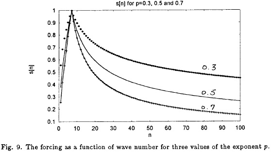
The -3 law for the logarithmic distribution of the kinetic energy in wave number space is found only when one considers the averaged kinetic energy for considerable lengths of time intervals. On individual days considerable deviations may be found. We should therefore also consider the specification of the forcing S[n] given in (2.4) as such an time-averaged distribution. It is thus of interest to investigate the logarithmic slope for other distributions of S[n]. Figure 9 shows three examples of distributions obtained by varying the exponent (p) from the value of p = 1/2 used in the above considerations. It is noticed that a smaller value of p results particularly in larger values of the forcing for the larger wave numbers, while the opposite is the case for larger values of p. Varying p by 0.05 from 0.3 to 0.7 the logarithmic slopes of the kinetic energy have been calculated for the small and the large wave numbers. The results are listed in Table 1 where the slopes are given separately for the long (L.W.) and the short waves (S.W.).

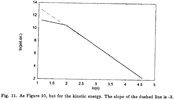
It is thus seen that for each change of p by +0.05 the two slopes will change by 0.1 for the long waves and -0.1 for the short waves. As stated above the logarithmic slope of the available potential energy is about -2.5 in the example used for the figures so far. It is, however, possible to approximate a logarithmic slope of about -3 for both the eddy available potential energy and the eddy kinetic energy. After some numerical experimentation it was found that p = 0.56 results in the desired slope for the eddy available potential energy and as the Table shows the eddy kinetic energy will then have a slope of about -3.1. Figure 10 shows the distribution of the eddy available potential energy. The dashed line has the slope of-3. Figure 11 displays in a similar way the eddy kinetic energy where the dashed line also has the slope of -3.

The investigation reported in this note is somewhat more general than the investigations based solely on the first equation of motion (Wiin-Nielsen, 1998). Considering only the steady state solutions in the earlier and the present investigations we find, however, in both investigations that the nonlinear cascade of the kinetic energy is important for the kinetic energy as a function of wave number. The balance is in the present model mainly between the energy conversion from eddy available potential energy to eddy kinetic energy and the conversion due to the cascade processes. The first of these processes is not present in the simpler models based on the first equation of motion only.

The equations for the present model may also be integrated in the time dependent case from a given initial state. Such integrations have been performed starting from an initial state close to the steady state. These integrations show first of all that the steady state is stable. In addition, they contain oscillations of the gravity wave type moving with a velocity close to c = ɸ^1/2 and thus having a period of T = L_s/(nc) where L_s is the maximum wavelength.

 

4. Conclusions

It has been demonstrated that the simple model of a homogeneous fluid with a free surface and with a specified forcing can result in logarithmic slopes of about -3 for both the eddy available potential energy and the eddy kinetic energy. The interval for which the two slopes are about -3 is found for wave numbers somewhat larger than the maximum forcing and smaller than the dissipation range.

 

REFERENCES

Barros, V. R. and A. Wiin-Nielsen, 1974. On quasi- geostrophic turbulence: A numerical experiment, J. Atmos. Sci., 31, 609-621.         [ Links ]

Charney, J. G., 1971. Geostrophic turbulence, J. Atmos. Set., 28, 1087-1095.         [ Links ]

Fjørtoft, R., 1953. On the changes in the spectral distribution of kinetic energy for two-dimensional nondivergent flow, Tellus, 5, 225-230.         [ Links ]

Horn, L. H. and R. A. Bryson, 1963. An analysis of the geostrophic kinetic energy spectrum of large-scale atmospheric turbulence, Jour. of Geophys. Res., 68, 1059-1064.         [ Links ]

Julian, P. R., W. M. Washington, L. Hembree and C. Ridley, 1970. On the spectral distribution of large-scale atmospheric kinetic energy, J. Atmos. Sci., 27, 376-387.         [ Links ]

Kao, S.-K., 1970. Wave number - frequency analysis spectra of temperature in the free atmosphere, J. Atmos. Sci., 27, 1000-1007.         [ Links ]

Kao, S.-K. and L. L. Wendell, 1970. The kinetic energy of the large-scale atmospheric motion in wave number, frequency space: Northern Hemisphere, J. Atmos. Sci., 27, 359-375.         [ Links ]

Kraichnan, R., 1967. Inertial ranges in two-dimensional turbulence, Phys. Fluid, 10, 1417-1423.         [ Links ]

Leith, C. E., 1968. Diffusion approximation for two-dimensional turbulence, Phys. Fluid, 11, 671-672.         [ Links ]

Leith, C. E., 1971. Atmospheric predictability and two-dimensional turbulence, J. Atmos. Sci., 28, 145-161.         [ Links ]

Lilly, D. K., 1969. Numerical simulation of two-dimensional turbulence, Phys. Fluid, Suppl. II, 240-249.

Merilees, P. E. and T. Warn, 1972. The resolution implication of geostrophic turbulence, J. Atmos. Sci., 29, 990-991.         [ Links ]

Steinberg, L., A. Wiin-Nielsen and C. H. Yang, 1971. On nonlinear cascades in the large-scale atmospheric flow, J. of Geophys. Res., 76, 8629-8640.         [ Links ]

Wiin-Nielsen, A., 1967. On the annual variation and spectral distribution of atmospheric energy, Tellus, 19, 540- 559.         [ Links ]

Wiin-Nielsen, A., 1998. On the spectral distribution of kinetic energy in large-scale atmospheric flow, Nonlinear Geophysics, 5, 187-192.         [ Links ]

Wiin-Nielsen, A. and C.-T. Chen, 1993. Fundamentals of atmospheric energetics, Oxford University Press, 376 pp.         [ Links ]