Recent numerical experiments on three-months extended and seasonal weather prediction with a thermodynamic model*

 

J. ADEM¹, V. M. MENDOZA, A. RUIZ, E. E. VILLANUEVA and R. GARDUÑO

Centro de Ciencias de la Atmósfera, UNAM, Circuito Exterior, CU, 04510 México, D. F., México. ¹ Member of "El Colegio Nacional"

 

RESUMEN

El modelo termodinámico del clima de Adem (ATCM) ha sido adaptado para llevar a cabo pronósticos numéricos a tres meses y estacionales. El modelo usa la rejilla estereográfica polar para el Hemisferio Norte del NMC, con 1977 puntos e intervalos de rejilla de 408.5 Km. La capacidad del modelo ha sido evaluada en la región de México para el periodo febrero 1981 a noviembre 1983 que incluye "El Niño" 1982-83 y, más recientemente con base en tiempo real, para el periodo "El Niño" de junio 1997 a agosto 1998. Los resultados muestran una buena habilidad al pronosticar las anomalías estacionales de temperatura y precipitación durante este periodo de "El Niño", que también confirma los resultados para "El Niño" de 1982-83. Durante todo el periodo de junio 1997 a agosto 1998, el modelo predijo temperatura del aire sobre la normal y precipitación bajo la normal, que están de acuerdo con las observaciones correspondientes a una persistente y severa sequía que afecto a la República Mexicana durante ese periodo. Los resultados muestran que las temperaturas del océano juegan un papel importante en las predicciones, y pueden sugerir que las temperaturas oceánicas sobre la normal en las regiones adyacentes del Pacífico Mexicano, asociadas a "El Niño" causan temperaturas del aire por arriba de la normal y precipitación por debajo de la normal, favoreciendo posiblemente la sequía en la República Mexicana.

 

ABSTRACT

The Adem thermodynamic climate model (ATCM) has been adapted to carry out three-month extended and seasonal numerical weather predictions. The model uses the Northern Hemisphere NMC polar stereographic grid with 1977 points and a grid distance of 408.5 km. The performance of the model has been evaluated for the period February 1981 to November 1983, which includes the "El Niño" 1982-83, and more recently in a real time basis for the "El Niño" period from June 1997 to August 1998 for Mexico. The results show good skill in predicting seasonally temperature and precipitation anomalies during this "El Niño" period, which also confirms the results for the "El Niño" 1982-83. During the whole period June 1997 to August 1998, the model predicted above normal air-temperature and below normal precipitation, in agreement with the observations, which corresponded to a severe persistent drought in Mexico that existed during that period. The results show that the ocean temperatures play an important role in the predictions, and it may be suggested that the above normal ocean temperatures in the Pacific Ocean regions contiguous to Mexico associated with "El Niño" produced the above normal surface air-temperature and the below normal precipitation possibly favoring the drought situation in Mexico.

 

1. Introduction

With the availability of electronic computers and adequate initial data, short range numerical weather prediction was initiated in the Institute for Advance Studies in Princeton, by the classical paper of Charney, Fj0rtoft and Von Neumann (1950), with relative success. Since that time with new generation of computers, better data, and improved models, daily predictions for about a week have been carried out, with some success.

In the short range prediction (1 to 2 days), the models are based mainly on the conservation of momentum equation, and the thermodynamic energy equation is used without heat sources and sinks. Therefore these models are considered dynamic. For extended prediction (one week) the heat sources and sinks become important and have to be added in the models.

For periods of time longer than a week, the predictability of the detailed daily weather becomes an impossible task. However, an attempt can be made to predict the average conditions over the considered period and predictability seems to increase for periods from a month to a season associated with the anomalies in the underlying surface. In fact, in the early sixties, in the Extended Forecast Division of the National Meteorological Center (NMC) of the United States, which was headed by the late Jerome Namias, subjective monthly predictions were carried out in which sea surface temperature (SST) and snow and ice anomalies were used.

A that time, the senior author developed the first energy balance model that used the Defant (1921) type "austausch" coefficient to parameterize the horizontal large scale turbulent transport associated with the synoptic scale cyclones and anticyclones (Adem, 1962, 1963). This model was adapted for monthly prediction, incorporating as initial conditions, the 700-mb temperature anomalies, the SST anomalies and the snow and ice anomalies (Adem, 1964a, 1965 and 1970b). Evaluation of the predictions of temperature over the contiguous U. S. and SST in the North Atlantic and Pacific oceans showed an encouraging skill (Adem, 1964a, 1964b, 1965, 1970b; Adem and Jacob, 1968).

In the eighties experiments were carried out in the Lamont Geological Laboratory of Columbia University by a group headed by the late William Donn, resulting in an improvement in the skill of the predictions (Adem and Donn, 1981; Donn et al, 1986). Furthermore, in the former Soviet Union, Mamedov (1986, 1989) carried out predictions of surface temperature using a thermodynamic model, with some success. The influence functions calculated by Marchuk and Skiba (1976) showed the feasibility of predicting the monthly mean surface temperature anomalies with a thermodynamic model.

Recently experiments were carried out in the Center of Atmospheric Sciences of the National University of Mexico to verify the monthly predictions of 700-mb and surface air-temperature anomalies, as well as the precipitation anomalies over Mexico, but instead of using the original abridged NMC grid of 817 km and 512 points, the original NMC grid of 408.5 km and 1977 points was used, which is more adequate for countries as Mexico (Adem et al, 1995b).

In the present paper an attempt has been made to extend the period of prediction to three months instead of only one, and carry out also seasonal predictions.

The monthly extended and seasonal predictions were carried out for the period from February 1981 to November 1983, which included an "El Niño" period. These results were reported in the W. M. O. Workshop on Dynamic Extended-Range Forecast in Toulouse, France, 17-21 November, 1997 (Adem et al.,1997). Furthermore, predictions for the most recent "El Niño" period 1997-98 were carried out and are also reported here.

 

2. Description of the model

The model (Adem, 1970b, 1979, 1991) consists of an atmospheric layer of 9 km thickness, including a cloud layer, an upper ocean layer of 60 meters in depth, and a continental layer of negligible depth. It also includes a layer of ice and snow over the continents and oceans. The thermodynamic energy equation is applied to the atmosphere-ocean-continent system described above.

Time averaging of the variables of the order of one month is used; and it is assumed that the hydrostatic equilibrium, perfect gas and continuity equations, as well as the geostrophic balance equations used for the horizontal wind, are valid for the time-averaged variables. Therefore, the vertically integrated equation of thermal energy for the atmospheric layer is the following:

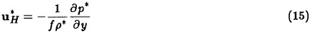
Where ∇ is the two-dimensional horizontal gradient operator; T'_m is the departure of the mean atmospheric temperature from a constant value T_m0, where T_m0 >> T'_m; c_v is the specific heat of air at constant volume; and p_m and V_m, given by:

and

are respectively the mean density and the horizontal velocity of the mean wind in the troposphere; H is the constant height of the model atmosphere and ρ* is the density field. V*_H is the horizontal vector of the velocity of the wind and K is the horizontal austausch coefficient for the atmosphere.

On the right hand side of equation (1), E_T is the rate of heating by short and long wave radiation, G₅ is the rate of heating by condensation of water vapor in the clouds, and G₂is the rate of heating by vertical turbulent transport from the surface.

On the left hand side, ρ_mc_vH∂T'_m/∂t is the local rate of change of thermal energy, and ρ_mc_vHV_m ⋅ ∇T'_mand −ρ_mc_vHK∇²T'_m are the rates of change by advection of thermal energy, by mean wind and by large-scale horizontal eddies, respectively.

The thermal energy equation for the upper layer of the ocean (Adem, 1970a) is the following:

Were T'_s is the departure of the SST from a constant value T_s0,T_s0 >> T'_s;ρ_s is a constant density and c_s is the specific heat; h is the depth of the layer V_ST is the horizontal vector of the velocity of the mean ocean currents in the layer; and K_s is the constant austausch coefficient for the ocean upper layer.

On the right hand side of equation (2), E_s is the rate of heating by short and long wave radiation; G₂ is the rate of sensible heat given off to the atmosphere by vertical turbulent transport; and G₃ is the rate at which the heat is lost by evaporation.

On the left hand side, ρ_sc_sh∂T'_s/∂t is the local rate of change of thermal energy, and ρ_sc_shV_ST ⋅ ∇T'_s and −ρ_sc_shK_s∇²T'_s are the advections of thermal energy by mean ocean currents and by large-scale horizontal eddies, respectively.

In the continents, the equation (2) is reduced to:

0 = E_s + G₂ + G₃ (2')

 

2.1 Parameterization of the heating functions

The parameterization of the heating by short and long wave radiation in the atmosphere (E_T) and at the surface (E_S) is carried out assuming that the cloud layer and the surface of the Earth radiate as black bodies and that the clear atmosphere has a window for wavelengths between 8 and 12 microns and that the current content of atmospheric CO₂ affects the emission for wavelengths between 12 and 14 microns and between 16 and 18 microns (Adem and Garduño, 1982). Furthermore, the Savino-Ånström formula is used for the absorption of the short-wave radiation at the surface of the Earth (Budyko, 1956).

The resultant formulas, linearized with respect to T'_m and T'_s are the following:

where F₃₀, F'₃₀, F₃₁, F₃₂, F'₃₂, F₃₄, F'₃₄, F₃₅ and F₃₆ are constant; ε is the cloud cover and ε_N is the corresponding normal value; a₂ and b₃ are functions of the latitude and the season; (Q + q)₀ is the total radiation received by the surface with clear sky; k is a function of latitude; I is the insolation and α the surface albedo.

Another alternative for the oceans, is the use of the non-linear formula for E_s (Adem, 1962) given by:

where T_a is the ship-deck temperature; σ = 5.6697 × 10⁻⁸watt m⁻² K⁻⁴ is the Stefan-Boltzman constant; T_C2 is the temperature at the bottom of the layer of clouds, considered as a constant; and E(T*) = σT*⁴ − F(T*) is the energy per unit area per unit time emitted by a horizontal boundary with temperature T* of an atmospheric layer, the function F(T*) represent the energy per unit area per unit time which is not absorbed by the atmospheric layer (Adem, 1962).

For the rates at which heat is added to the atmosphere by vertical turbulent transport from the surface (G₂) and heat is lost by evaporation at the surface (G₃) we use over the oceans the formulas (Jacobs, 1951):

where K₃ and K₄ are constants, |V_a| is the ship-deck wind speed; e_s(T_s) and e_s(T_a) are the saturation vapor pressure corresponding to the SST and the ship-deck air temperature, respectively; and U is the ship-deck air relative humidity.

Another alternative is the use of the linearized approximate formulas deduced by Clapp et al. (1965), adequate for use in the simpler linearized version of the model, which are the following:

where G_2N ,G_3N ,T'_SN and T'_mN are the normal values of G₂, G₃, T'_S and T'_m respectively; B is a constant; U_N is the normal value of the surface relative humidity (Adem, 1970a); and |V_aN| is the normal surface wind speed.

In the continents we use for G₂ a similar formula to that over the oceans and for G₃ the formula:

where d₇ is a seasonal value that depends on the map coordinates and, E_SN is the normal value of E_S (Clapp et al, 1965).

For the heat gained by condensation of water vapor in the clouds, we use the following empirical formula deduced also by Clapp et al (1965):

where G_5N is the normal seasonal value of (G₅), b, d" and c" are function of x and y that vary with the season.

The cloud cover is considered as a variable and is given by:

ε = ε_N + D₂(G₅ - G_5N) (11')

where D₂ is an empirical constant (Clapp et al, 1965).

 

2.2 Parameterization of the advection by mean winds and by ocean currents

The advection of thermal energy by mean wind in the atmospheric layer of the model (denoted by AD) is defined by:

where for the horizontal velocity of the wind (V*_H), we will use, as in a previous paper (Adem, 1970b), the following expression:

where V*_N0b is the velocity of normal observed wind, V* is the predicted horizontal velocity of the wind, and V*_N is the computed normal horizontal velocity of the wind. Substituting equation (13) in equation (12), we obtain:

In equation (14) the components of V*_Nob, V* and V*_N are computed using the geostrophic wind formulas given by:

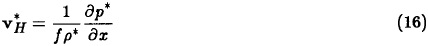
where u*_H and v*_H are the x and y components of V*_Hand ƒ is the Coriolis parameter.

In the model the temperature field is given by:

where Γ is the constant lapse rate for the standard atmosphere of mid-latitudes and T_m = T_m0 + T'_m is the mean temperature in the troposphere.

Using equation (17) together with the equation of hydrostatic equilibrium and perfect gas, we obtain

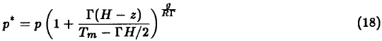
and

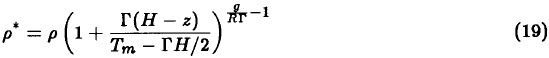
where, p and ρ are respectively the values of the pressure and density at z = H, g is the acceleration of gravity and R is the gas constant.

In this way, the components of V*_Nob are computed substituting equations (18) and (19) in the geostrophic wind formulas (15) and (16). The resulting formulas are

and

where u*_Noband v*_Nobare the x and y components of V*_Nob, p_Noband T_mNob are the corresponding normal values of p and T_m, respectively and T*_Nob= Γ(z − H/2) + T_mNob.

In the model, p_Noband T_mNob are computed using 700-mb data, from the following formulas:

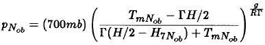
and

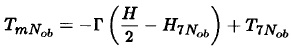
where T_7Nob and H_7Nob are the observed normal 700-mb temperature and height, respectively.

The components of V* are computed also substituting equations (18) and (19) in the geostrophic wind formulas (15) and (16), but in this case using the perfect gas equation and assuming that the density at the top of the atmospheric layer (z = H) is a constant (Adem, 1967). The resulting formulas are:

and

Similar formulas are obtained for V*_N. Substituting equations (19), (20), (21), (22), (23) and the formulas for V*_N in equation (14), we obtain, for the advection of thermal energy by mean wind, the following formula:

where J is the Jacobian operator and where

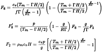
and

In the normal case, the last term on the right-hand side of formula (24) is equal zero. For its use in the model, formula (24) is replaced by:

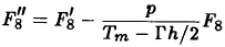
where (F₈)₀, (F'₈)₀ and (F''₈)₀ are obtained from the above formulas using the constant T_m0 and p₀ instead of T_m and p; where p = p₀ + p' and where p' << p₀.

Formula (25) is a linear function of ∂T'_m/∂x and ∂T'_m/∂y, and corresponds to the option 3 used in a previous work (Adem, 1970b), the sum of the first two terms on the right-hand side gives the advection by the prescribed observed normal wind, and the last term represents the advection of thermal energy by the anomalies of the wind predicted by the model.

The option used in this work is obtained from the linearization of equation (14) and is given by the following equation:

In this case, we obtain:

In the normal case, the terms with (F'₈)₀ on the right-hand side of equation (27) are equal to zero.

For the horizontal ocean currents in the mixed layer we shall assume that:

where V_SW is the horizontal normal seasonal ocean velocity in the layer, V_S is the velocity of the resultant pure wind drift ocean current in the layer and V_sN is the corresponding normal value of V_s.

To evaluate V_s we shall use the classical Ekman's formulas for a pure wind drift current. Therefore, the components of the ocean current in the layer will be expressed by (Adem, 1970a):

where φ is the latitude; u_s and v_s, the x and y components respectively, of the resultant velocity of the pure drift current in the layer of depth h; and u₀ and v_a, the x and y components of the surface wind respectively. The range of values of C₁ and θ are limited to 45° ≤ θ ≤ 90° and 0.235 ≤ C₁≤1.

For θ = 45° and C₁ = 1 we have the resultant pure drift current in a very shallow layer. For θ = 90° and C₁= 0.235 we have the resultant pure drift current in the Ekman layer.

Namias (1959, 1965, 1972); Eber (1961); Jacob (1967); Clark (1972); and Adem (1970a, 1975) have made estimates of changes in SST anomalies, due to advection by mean ocean currents. The relation that they use to evaluate the ocean currents corresponds to the case C₁= 1 and θ = 45°.

Formulas (29) and (30) correspond to the case |V_a| > 6 m s⁻¹, where |V_a| is the ship-deck wind speed. For |V_a|≤ 6 m s⁻¹ we have used the factor 0.0259/ instead of 0.0126 (Adem, 1970a). The normal wind drift current V_sN is computed from the normal values of the surface wind with formulas (29) and (30).

According with (28) the advection by mean ocean current can be expressed by:

The term ρ_sc_shV_SW · ∇T'_s is the thermal energy advection by normal seasonal ocean current and the term ρ_sc_sh(V_S − V_SN) · ∇T'_s is the thermal energy advection due to the anomaly of the wind drift ocean current. According to Frankignoul (1985), the surface currents act mainly by distorting the normal SST gradient, because over most of the oceans ∇T_sN >> ∇(T_S − T_sN), where T_sN is the normal value of T_s and (T_s − T_sN) is the SST anomaly. This is in agreement with Namias (1959), Eber (1961), Jacob (1967) and Adem (1970a), who showed that in the term (V_S − V_SN) · ∇T'_s, (V_S − V_sN) · ∇(T_S − T_sN) can be neglected. Therefore in the terms(V_S − V_SN) · ∇T'_s and V_SW · ∇T'_s of equation (31) we shall prescribe the normal SST gradient using ∇T_sN0b instead ∇T_s, where ∇T_sN0bis the observed normal SST.

 

2.3 The integration of the model

In the model used up till now, we have made the following assumptions:

I. In equation (1) the advection by mean wind is taken as zero or as advection by a prescribed normal mean wind.

II. In equation (2), the horizontal transports of thermal energy by mean ocean currents and by turbulent eddies are neglected.

III. Equations (1) and (2) are integrated using an implicit scheme, therefore the terms ∂T'_m/∂t and ∂T'_s/∂t are replaced by (T'_m -T'_mp)/Δt and (T'_s -T'_sp)/ΔT, respectively, where T'_mp and T'_sp are the corresponding values of T'_m and T'_s in the previous month and Δt is the time interval taken as a month, this large time interval is possible due to the implicit scheme of integration used in the model.

Substituting the parameterized heating functions (3), (4), (8), (9), (10), (11) and (11') in equations (1) and (2), and using assumptions I, II and III, we obtain two linear equations to compute T'_m and T'_s. Due to assumption II, equation (1) becomes algebraic, yielding the surface temperature as a function of the mean temperature in the troposphere (Adem, 1965) given by

where F₇₂, F₇₃, F₇₅, F₇₆ and F₇₇ are known functions of the map coordinates x and y (Adem, 1965). The surface temperature in (32) is a linear function of the mean temperature in the troposphere and, due to formula (11), it is also a linear function of the spatial derivatives of the mean temperature in the troposphere. In the normal case, the last three terms on the right-hand side of equation (32) are equal to zero.

The surface temperature given by (32) is substituted in the equation (1) for the atmosphere, and we obtain an elliptic differential equation of the type:

where F, F', F'' and F''' are known functions of the map coordinates x and y (Adem, 1965).

The assumptions I, II and III have reduced the integration problem to the solution of a linear second-order elliptic differential equation, in which the mean temperature in the troposphere obtained from (33) is substituted in equation (32) to compute the surface temperature.

Adem (1970b) introduced a method that permits to remove the assumptions I and II and still get the same type of integration problem. In this work we use the same method of which a brief summary will be give here.

Considering that the oceanic mixed layer has a large storage capacity of thermal energy, the term ρ_sc_sh∂T'_s/∂t is larger than any of the other terms in equation (2), and therefore we can attempt to solve it with forward or centered differences. The numerical field of the surface ocean temperature obtained from equation (2) by means of this explicit scheme is substituted in equation (1), in which we still use backward differences. This is done because in contrast with what happens in the ocean the storage term in the atmosphere is small compared with the heating functions and, therefore, in the integration of equation (1), an implicit scheme should be used. The integration problem is therefore reduced again to the solving of an elliptic differential equation for the mean temperature in the troposphere.

The integration of equation (2) with forward or centered differences permits us, in addition to removing the assumption (2), to use the non-linear formulas (5), (6) and (7) for the heating functions in the oceans. However in equation (2'), we still use the linear formulas (4), (8) and (10) for the heating functions and in the continents the surface temperature is given by (32).

Since formula (27), used in this work, is a linear function of ∂T'_m/∂x and ∂T'_m/∂y, its use in equation (1), together with the linear formulas for the heating functions, yields and equation of the same type as equation (33).

The spatial integration of the model is performed over the Northern Hemisphere with the use of the NMC grid of 1977 points with 408.5 km resolution and the equation (33) is solved prescribing T'_m at the closed boundary using a relaxation method.

 

3. Numerical predictions

We carry out monthly predictions of surface and 700-mb temperature anomalies and precipitation anomalies for extended periods as long as three months, as well as seasonal predictions in the Northern Hemisphere. The procedure used in the prediction of the first month consist in making a prediction for the normal values, using observed normal values of the previous month as initial conditions and another prediction for the given month using the observed values of the previous month as initial condition (normal plus anomaly). The predicted anomaly for the first month is obtained by subtracting from the computed values the corresponding computed normal values. The procedure used for the prediction of the second and third month is similar to the one used in the first, but instead of using the observed values of the previous month as initial conditions we use the predicted values of the previous month.

 

3.1 Prediction for the period February 1981 to November 1989

We carry out monthly extended and seasonal predictions for the period of 32 months, from February 1981 to November 1983, which includes an "El Niño" period. The monthly predictions are overlapping in two months, so that we obtain 32 three-months overlapping periods which give a total of 96 cases of monthly predictions. When the predicted three-month period coincides with the three months of a season, then we obtain a seasonal prediction with the average from the three predicted months in the season.

In these prediction experiments, the SST anomalies are predicted from equation (2), using forward finite differences with time intervals of one day, so that for each monthly prediction 30 time steps are required.

For the heating functions in equation (2), we use the non-linear formulas (5), (6) and (7), in which due to the lack of available data, we use seasonal normal values for the cloud cover and for the ship-deck wind speed. For the surface air-temperature (T_a) and the surface relative humidity (U) we have computed as in a previous paper (Adem et al, 1994), the anomalies of these variables using available data of 850-mb temperature and the following formulas:

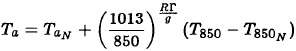
and

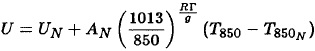
where T_aN is the observed normal value of T_a; T₈₅₀ is the temperature at 850-mb level and T_850N is the corresponding normal value of T₈₅₀; U_N is the observed normal value of U and A_N is given by:

In formulas (29) and (30) we use C₁ = 0.235, which corresponds to the resultant pure wind drift current in the whole frictional ocean layer, and θ equal to zero degrees corresponding to the case in which the wind drift current has the same direction as the wind. For the horizontal normal seasonal ocean velocity in the layer, we assumed that V_SW = C₁V_S0 where V_S0 is the horizontal normal seasonal ocean velocity observed in the surface obtained from the available data of NCAR network. The components of the surface wind in equation (29) and (30) are computed from formulas (15) and (16), assuming geostrophic wind and that the density at z=0 is a constant, therefore the surface wind in equations (29) and (30) can be computed from available data of atmospheric sea surface pressure. The constant Austausch coefficient K_s is equal to 1 × 10⁴m²s⁻¹ (Adem et al, 1995a).

The boundary conditions for equation (2) are described in detail in a previous work (Adem, et al. 1995a) and the initial conditions for the first month of prediction are: the monthly SST, the air-temperature of the 850-mb level and the atmospheric sea surface pressure observed in the previous month. The atmospheric initial conditions are maintained fix through the three-month period of prediction, so that equation (2) can be integrated independently of the atmospheric equation (33).

The boundary conditions for equation (33) and the relaxation method for its solution are described in a previous work (Adem, 1964a), and the initial conditions for the first month of prediction are: the air-temperature at the 700-mb level observed in the previous month and the albedo based on the snow and ice distribution in the last week of the previous month. The corresponding ocean surface temperature anomalies predicted by equation (2) are used as external forcing in the atmospheric equation (33) in each month of prediction. The constant Austausch coefficient for the atmosphere, K, is equal to 3 × 10⁶m²s⁻¹ this value correspond to the scale of migratory cyclones and anticyclones of the middle latitudes.

The SST values and the corresponding normal values were obtained from the National Weather Service-NOAA. The atmospheric surface pressure and 850 and 700-mb temperature and their corresponding normal values were obtained from the NCAR NMC grid points data set. The snow and ice data have been prepared by NESS-NOAA, and the data of normal albedo maps have been prepared by Donn and Adem (1981).

In previous applications the surface albedo has influenced the predictions through the variations in snow and ice, and in this way important anomalies have been predicted in middle latitudes, as has been verified over the contiguous US (Adem, 1965; Adem and Donn, 1981). It is evident that the influence of the snow and ice effect decreases towards the lower latitudes, therefore in the experiments described in this paper we have neglected such effect in Mexico.

The precipitation anomalies are predicted in the model from formula (11) assuming that they are proportional to the anomalies of heat gained by condensation of water vapor in the clouds, which are computed internally in the model, and therefore interact with the temperature field.

To show the effect of the SST in the seasonal predictions, we illustrate as example, in Figure 1, the surface temperature anomalies predicted for the summer 1982, in tenths of Celsius degrees, for the quarter of the integration region which includes Mexico. Figure 1A shows the predicted anomalies when the storage of thermal energy in the atmosphere is included and where the 700-mb temperature anomalies in May of 1982 are used as initial condition and the SST anomalies predicted with equation (2), are used as forcing. Figure 1B shows the predicted anomalies without the atmospheric storage, and where only the SST anomalies are used as forcing.

Figure 1A and Figure 1B are for practical purposes identical, showing that the storage of thermal energy in the atmosphere can safely be neglected in the seasonal prediction and that the SST anomalies play the most important role in the prediction. It is interesting to notice that the positive temperature anomalies of the Pacific and Atlantic oceans are associated with important positive anomalies in Mexico, for example the isothermal of 0.5 °C penetrating deeply from both oceans to the Mexican territory.

The results for the summer 1982 over Mexico are shown in the next three figures. Figure 2 shows in part A the predicted anomalies of surface ground temperature (°C) and part B the observed surface air temperature anomalies. Figure 3 shows the 700-mb temperature anomalies, in Celsius degree, predicted by the model (part A), and observed (part B). Figure 4 shows the sign of the precipitation anomalies computed (part A) and observed (part B).

From Figures 2, 3 and 4 we see that, for the summer 1982, the sign of the predicted anomalies is predominantly positive for temperature, and negative for precipitation. This particular summer, when heat and drought conditions over Mexico existed, the signs have been correctly predicted, as can be seen by comparison of parts A with parts B.

Two verification tests were used for the extended predictions of 700-mb temperature and precipitation anomalies over Mexico. In the first one, the results were verified simply for the prediction of the correct sign of the anomalies. The skill of these results was determined with the formula used by Adem and Donn (1981):

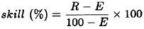
where R and E are the percentages of signs correctly predicted by the model and by persistence, respectively. In the second verification, we use, from the WMO standardized system, the root mean square skill score in percentage, given by:

where RMSE is the root mean square error. The prediction by persistence is equal to the observed anomaly in the last month of the previous three-months period, changing in each three-months period. For example, the prediction by persistence for the period June-July-August is equal to the observed anomaly of May, namely that, the anomaly of May is compared with those for June, July and August.

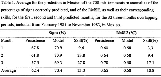
Table 1 shows, for the 700-mb temperature anomalies, the average of the percentage of signs correctly predicted and the RMSE, as well as their corresponding skill for the first, second and third month, obtained from the 32-months period, February 1981 to November 1983, in Mexico. This table shows that the percentage of signs correctly predicted by the model remains practically the same from the first to the third month, while the corresponding percentage of persistence decreases from 67.8% for the first month to 57.5% for the third month, so that the skill of the model increases from 9.6% for the first month to 27.8% for the third month. On the other hand, the RMSE of the model remains constant with a value of 0.58 °C from the first to the third month, while the RMSE of persistence changes from 0.60 for the first month to 0.70 °C for the third month, so that the skill of the model increases from 3.3% for the first month to 17.1% for the third one.

The seasonal average of the percentage of signs of the monthly 700-mb temperature correctly predicted and the RMSE, in Celsius degrees, as well as the corresponding skills over persistence are shown in Table 2, which shows that for the whole period, the model predicts correctly 70.2% of the signs, while persistence predicts correctly 62.4%, and therefore the skill of the model is 21.0%. This table shows also that for the whole period the RMSE of model is 0.58 °C while persistence is 0.65 °C, so that the skill of the model is 10.8%.

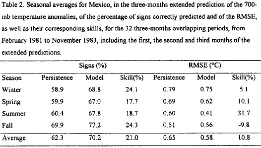
Table 3 is similar to Table 2 but in this case for the precipitation anomalies. For the whole period, the model predicts 52.4% of the signs, which is the same than persistence and therefore the skill is zero, on the other hand the RMSE of the model for the whole period is 40.5 mm per month, which is 13.5 mm per month lower than the RMSE of persistence, so that the skill of the model is 25.0%. Table 3 shows that the worst three-months extended predictions of the model occurs during spring and the best predictions occurs during winter.

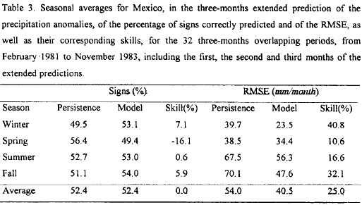
Table 4 is as Table 3 except that in this case we only consider the "El Niño" period, which consists of the 23 months from November 1981 to November 1983. Comparison of Table 4 with Table 3 shows that the skill of the model for the "El Niño" period is better than the one for the whole 32 months-period, and that the prediction of the precipitation anomalies for summer increases substantially in the "El Niño" period. Table 4 shows also that the best skill in predicting the sign of the anomaly is obtained in the summer, which is the rainy season in Mexico. This result is in agreement with a previous paper on the monthly prediction for Mexico (Adem et al., 1995b).

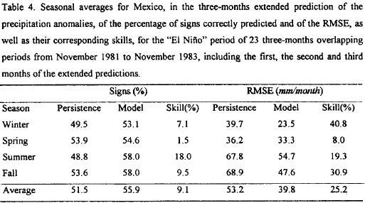
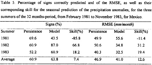
Table 5 shows the percentage of signs correctly predicted of the precipitation anomalies and the RMSE, as well as the corresponding skill for the three summers of the 32 months-period, in Mexico. The seasonal field is obtained with the average of the three monthly fields in the season. In this case, the prediction by persistence is equal to the observed precipitation anomalies of the previous season (spring). Table 5 shows that the worst predictions of the model is for the summer of 1981, when the skill in signs and the skill in RMSE are negatives (-85.8% and -11.4%, respectively), however for the summers 1982 and 1983 the model is better than persistence. This result suggests that the model has some good skill in predicting the precipitation anomalies for Mexico in the rainy season during a period of strong "El Niño".

 

3.2 Prediction for the El Niño 1997-98

Due to the fact that the previous results suggest that SST anomalies play the most important role in the seasonal prediction over Mexico during the period of El Niño 1982-83, we used in the recent experiment for "El Niño" 1997-98 the simplest version of the model with surface ocean temperature anomalies as the only initial condition. In this version of the model, we take into account the assumptions (2) and (3) of the section 2.3 and therefore we use the linear formulas for the heating functions. For the advection of thermal energy by mean wind we use, as in the previous experiments, the linear equation (27). The surface temperature, given by the equation (32), is computed internally in the model and depends strongly on the SST of the previous month contained in the storage of thermal energy in the oceans.

The experiments were carried out on real time basis using data of SSTA from NOAA/NESDIS 50-km Global Analysis and the observed surface air temperature anomalies and observed precipitation anomalies in Mexico, were obtained from NOAA/CIRES Climate Diagnostic Center, Boulder Colorado.

The seasonal prediction experiments on real time for summer and fall 1997, winter 1997-98, spring and summer 1998 are shown in the Figures 5, 6, 7, 8 and 9, respectively. The comparison between Part A (predicted) and Part B (observed) of these figures, shows that for the summer and fall 1997 and spring and summer 1998 (Figs. 5, 6, 8 and 9) the model predicts reasonably well the sign and size of the persistent positive anomalies of the surface air temperature (except during the winter 1997-98) during the long period of "El Niño" 1997-98. The corresponding predictions of the sign of the anomalies of precipitation in Figures 10, 11, 12, 13 and 14 show that the model was generally able to predict the persistence of the drought through the 5 seasons of the "El Niño" 1997-98 in Mexico.

 

4. Conclusions

1. The experiments of the monthly prediction for extended periods as long as three months for the 32-months period verified over Mexico show good skill in predicting correctly the size and the sign of the 700-mb temperature anomalies. However, the skill of the model in predicting correctly the size of the anomalies (RMSE skill score) is lower than the skill of the model in predicting correctly their sign.

2. The best skill, in predicting the sign of the precipitation anomalies, in the three-months extended prediction, is obtained during the "El Niño" period (from November 1981 to November 1983), and the worst skill is obtained during the non "El Niño" period (from February to October 1981).

3. The results show that the storage of thermal energy in the atmosphere can safely be neglected and that the SST anomalies play the most important role in these predictions over Mexico. The monthly predictions presented in a previous paper, also showed a strong dependence on the SST anomalies (Adem et al, 1995b).

4. The experiments suggest that warm waters in the Pacific Ocean regions contiguous to Mexico, which were present in the strong "El Niño" and Southern Oscillation (ENSO) of 198283, could possibly produce above normal temperatures and below normal precipitation, favoring a drought situation in Mexico, with the possibility of predicting it with the model for extended periods as long as three months or a season. This has been confirmed with the seasonal predictions in the most recent period of "El Niño" from the summer 1997 to the summer 1998. However, we cannot generalize this conclusion, because we are dealing with a small number of cases, which are included in a period of strong ENSO. Therefore more experiments for other ENSO and non-ENSO years are needed to generalize this suggestion.

 

4.1 Advantages, limitations and future developments of the model

1. The model allows an easier incorporation of the heating functions, and of the surface interactions.

2. In the integration the time-steps are of a period that varies from one day to one month, depending on the type of experiment. This allows to run experiments, in the much shorter time than the general circulation models.

3. The transports by mean wind and by ocean currents are included in a crude way in the present model. An attempt is been made currently to compute explicitly the wind and the ocean current using the vorticity equation coupled with the thermodynamic energy equation (Mendoza, 1993).

4. The parameterization of the turbulent transport, is an important research topic. At present, we use an Austausch coefficient of Defant type, which is of the order of 3 × 10⁶m²s⁻¹ in the atmospheric layer and of 1 × 10⁴m²s⁻¹ in the oceanic layer.

5. The present model includes only a 9 km layer in the atmosphere, a 60 meters fully mixed layer in the ocean, an a continental layer of negligible depth, and covers only the Northern Hemisphere up till about 10°N, using the NMC stereographic projection grid. It is recommended to develop a multiple layer model including the Stratosphere and the Thermocline with adequate flows of heat, momentum and mass between contiguous layers.

6. The model may also be developed as a global one, to be able to include more adequately the interactions near the equator, such as the "El Niño" events. This also would allow to carry out experiments related to the Southern Hemisphere.

 

Acknowledgements

We are indebted to Jorge Zintzun, Alejandro Aguilar and Berta Oda for the computational technical support and Ma. Esther Grijalva for the final preparation of the manuscript, and Thelma del Cid for the final technical revision of the manuscript.

 

REFERENCES

Adem, J., 1962. On the theory of the general circulation of the atmosphere, Tellus, 14, 102-115.         [ Links ]

Adem, J., 1963. Preliminary computations on the maintenance and prediction of seasonal temperatures in the troposphere. Mon. Wea. Rev., 91, 375-396.         [ Links ]

Adem, J., 1964a. On the physical basis for the numerical prediction of monthly and seasonal temperatures in the troposphere-ocean-continent system. Mon. Wea. Rev., 92, 91-104.         [ Links ]

Adem, J., 1964b. On the normal thermal state of the troposphere-ocean-continent system in the Northern Hemisphere. Geofís. Int., 4, 3-32.         [ Links ]

Adem, J., 1965. Experiments aiming at monthly and seasonal numerical weather prediction. Mon. Wea. Rev., 93, 495-503.         [ Links ]

Adem, J., 1967. Relation among wind, temperature, pressure and density, with particular reference to monthly averages. Mon. Wea. Rev., 95, 531-539.         [ Links ]

Adem, J., 1970a. On the prediction of mean monthly ocean temperature. Tellus, 22, 410-430.         [ Links ]

Adem, J., 1970b. Incorporation of advection of heat by mean winds and by ocean currents in a thermodynamic model for long-range weather prediction. Mon. Wea. Rev., 98, 776-786.         [ Links ]

Adem, J., 1975. Numerical-thermodynamical prediction of mean monthly ocean temperatures. Tellus, 27, 541-551.         [ Links ]

Adem, J., 1979. Low resolution thermodynamic grid models. Dyn. Atmos. Oceans., 3, 433-451.         [ Links ]

Adem, J., 1991. Review of the development and applications of the Adem thermodynamic climate model. Climate Dynamics, 5, 145-160.         [ Links ]

Adem, J. and W. L. Jacob, 1968. On year experiments in numerical prediction of monthly mean temperature in the atmosphere-ocean-continent system. Mon. Wea. Rev., 96, 714-719.         [ Links ]

Adem, J. and W. Donn, 1981. Progress in monthly climate forecasting with a physical model. Bull. Amer. Met. Soc., 62, 1666-1675.         [ Links ]

Adem, J. and R. Garduño, 1982. Preliminary experiments on the climatic effect of an increase of the atmospheric C02, using a thermodynamic model. Geofís. Int., 21, 309-324.         [ Links ]

Adem, J., E. E. Villanueva and V. M. Mendoza, 1994. Preliminary experiments in the prediction of sea surface temperature anomalies in the Gulf of Mexico. Geofís. Int., 33, 511-521.         [ Links ]

Adem, J., V. M. Mendoza and E. E. Villanueva, 1995a. Numerical prediction of the sea surface temperature in the Pacific and Atlantic oceans. Geofís. Int., 34, 149- 160.         [ Links ]

Adem, J., A. Ruiz, V. M. Mendoza, R. Garduño and V. Barradas, 1995b. Recent experiments on monthly weather prediction with the Adem Thermodynamic Climate Model, with especial emphasis in Mexico. Atmósfera, 8, 23-34.         [ Links ]

Adem J., V. M. Mendoza, A. Ruiz, E. E. Villanueva and R. Garduño, 1998. Monthly extended and seasonal prediction with a thermodynamic model and its verification in Mexico. WMO International Workshop on Dynamical Extended Range Forecasting; Toulouse, France, 17-21 Nov., 1997. PWPR Report Series, Project No. 11, WMO/TD881, xi, 241p.         [ Links ]

Budyko, M. I., 1956. "Teplovoi balans zemnoi poverkhnosti" (The heat balance of the Earth's surface). Hydrometeorological Publishing House, Leningrad, 254 pp. (Translated from the original Russian by N. A. Stepanova, U. S. Weather Bureau, 1958).         [ Links ]

Charney, J. G, Fjörtoft, R. and J. Von Neumann, 1950. Numerical integration of the barotrophic vorticity equation, Tellus, 2, 237-254.         [ Links ]

Clapp, P. F., S. H. Scolnick, R. E. Taubensee and F. J. Winninghoff, 1965. Parameterization of certain atmospheric heat sources and sinks for use in a numerical model for monthly and seasonal forecasting. Internal Report, Extended Forecast Division (Available on request to Climate Analysis Center, NWS/NOAA, Washington, D.C. 20233).         [ Links ]

Clark, N. E., 1972. Specification of sea surface temperature anomaly patterns in the eastern North Pacific. J. Phys. Oceanogr., 2, 391-404.         [ Links ]

Defant, A., 1921. The Zirculation der atmosphare in den gemassigten Breiten der Erde. Geografiske Annaler, 3, 209-266.         [ Links ]

Donn, W. and J. Adem, 1981. Revised snow-ice normals from satellite observations. Proceedings of the 5th Climate Diagnostics Workshop, Seattle, Oct. 22-24, 1980, Washington, 144-152.         [ Links ]

Donn, W., R. Goldberg and J. Adem, 1986. Experiments in monthly temperature forecasting. Bull. Amer. Meteor. Soc., 67, 165-169.         [ Links ]

Eber, L. E., 1961. Effects of wind-induced advection of sea surface temperature. J. Geophys. Res., 66, 839-844.         [ Links ]

Frankignoul, C., 1985. Sea surface temperature anomalies, planetary waves and air-sea feedback in the middle latitudes. Rev. Geophys., bf 23, 357-390.         [ Links ]

Jacobs, W. C., 1951. The energy exchange between the sea and the atmosphere and some of its consequences. Bull. Scripps Inst, of Oceanography, Univ. of California 6, 27-122.         [ Links ]

Jacob, W. J., 1967. Numerical semiprediction of monthly sea surface temperature. J. Geophys. Res., 72, 1681-1689.         [ Links ]

Mamedov, A. S., 1986. Global thermodynamic model of forecast of mean monthly air temperature anomalies (January, February, August, September, October). Meteorologiya i Klimatologiya, No. 2 (170).         [ Links ]

Mamedov, A. S., 1989. Predicting mean monthly air temperature anomalies. Soviet Meteorology and Hydrology, 6, 31-38.         [ Links ]

Marchuk, G. I. and Yu. N. Skiba, 1976. Numerical calculation of the conjugate problem for a model of thermal interaction of the atmosphere with the oceans and continents. Izvestiya, Atmos. and Ocean. Physics, 12, 279-284.         [ Links ]

Mendoza, V. M., 1993. Un modelo termodinámico del clima. Tesis de Doctor en Física. Facultad de Ciencias, UNAM. México, D. F., 184 PP.         [ Links ]

Namias, J., 1959. Recent seasonal interactions between North Pacific waters and the overlying atmospheric circulation. J. Geophys. Res., 64, 631-646.         [ Links ]

Namias, J., 1965. Macroscopic association between mean monthly sea surface temperature and the overlying winds. J. Geophys. Res., 70, 2307-2318.         [ Links ]

Namias, J., 1972. Experiments in objectively predicting some atmospheric and oceanic variables for the winter of 1971-72. J. Appl. Meteorol., 11, 1164-1174.         [ Links ]

 

Nota

* Most of this paper was presented in the XXI General Assembly, The Hague, Holland, 19-23 April, 1999.