


 text new page (beta)
 English (pdf)
 Article in xml format
 Article references
 Send this article by e-mail
 Cited by SciELO
  Similars in
SciELO
Similars in
SciELO 
 Permalink
1. Introduction
Over time, inequality has been a topic that has worried researchers from different angles. According to the World Inequality Report 2018, economic inequality experienced, in recent decades, an increase in different regions of the world (Alvaredo et al., 2018). In addition, there is theoretical and empirical evidence that inequality can be transmitted from generation to generation.1 This has generated growing concern about the negative implications it may have on equal opportunities (Andrews and Leigh, 2009; Atkinson et al., 2011; Corak, 2013). In that sense, a generalized response argues that higher education is a potential mechanism that compensates for the implications of intergenerational transmission of socioeconomic (dis)advantages.2 With this in mind, one of the axes of education policy in many governments has been directed to invest a large amount of resources to expand higher education. Thus, its expansion can be associated with greater equal opportunities as greater potential is offered for the advancement of individuals from unfavorable environments (Blanden and Machin, 2004; Breen, 2010; Sturgis and Buscha, 2015).
However, the extent of expanding education to create equal opportunities is unclear. This depends on how new educational opportunities are distributed among different socioeconomic strata (Marginson, 2016). The empirical evidence that has been gathered in this regard has documented mixed results. For example, Breen et al. (2009) documented that educational expansion benefited more individuals from disadvantaged backgrounds in a sample of 9 European countries, thereby decreasing the inequality of educational opportunities. Blossfeld and Shavit (1993) analyzed 13 industrialized countries and showed that in 11 of the 13 countries analyzed, inequality of educational opportunities remained stable despite the dramatic educational expansion during the twentieth century. In contrast, Blanden and Machin (2004) found that the expansion of higher education in the United Kingdom disproportionately benefited individuals from relatively wealthy families. As a result, the expansion widened the participation gap in education between the rich and the poor. Likewise, Sturgis and Buscha (2015) found similar conclusions to Blanden and Machin (2004) for the case of England and Wales.
For the above, an obligatory question that arises is: how do level of schooling and intergenerational social mobility change under the expansion of higher education? This paper examines this question in Mexico, a case of study that is interesting at least for the following reasons. First, the empirical evidence gathered systematically places it as a country with low intergenerational social mobility, even when compared with countries in the Latin American region (Serrano and Torche, 2010; Vélez et al., 2013; Campos, 2016). Second, the construction of schools can be an important axis to analyze since, in Mexico, the literature finds that educational achievement correlates with socioeconomic conditions of origin. This relationship is accentuated at the extremes of the distribution; individuals who grow up in richer households are more likely to achieve greater schooling (Campos, 2016). Finally, in recent times, the Federal government decided to implement the program of Universities for Well-being Benito Juárez García. This program is based on increasing educational opportunities at the higher level for the most disadvantaged. It is intended to open 32 thousand spaces for students distributed in 100 new universities, a goal considered unprecedented in the Latin American region.
How can the expansion of higher education spaces generate profits in the education of individuals? The construction of new schools can induce changes in the decision of individuals to enroll either through the proximity or through the availability of the number of institutions. What lies behind this idea is that the proximity or availability of new educational spaces reduces the cost of education.3 For example, the presence of a new, closer educational institution may cause costs to be avoided when compared to a more distant institution, such as; lodging costs, travel costs and other non-monetary costs for living away from the family (Frenette, 2006; Spiess and Wrohlich, 2010; Kerr, 1991). In other words, the availability or location of educational institutions closer to individuals can be seen as an implicit subsidy to education (Kling, 2001).
The empirical evidence that has been gathered in that regard is consistent with the above. With regard to proximity, Card (1995) estimated the effect of education on income for a sample of men in the United States. To identify the effect, the author uses the geographical proximity of the universities in the county where the individuals lived at age 17 to instrument the schooling and found, among other things, that a shorter distance to the university increases the probability of attending school. Similarly, Doyle and Skinner (2016) estimated that the density of university opportunities has a statistically significant and positive impact on the accumulation of schooling. In the same vein, literature shows that the availability of educational spaces can generate an exogenous variation in individual decisions to attend school or not. For example, Duflo (2001) estimated the returns to education by exploiting a natural experiment that provided the program of massive construction of primary schools in Indonesia. Among other things, she showed that school building has a positive causal effect on the average schooling of Indonesian men. Specifically, she estimated that for every elementary school built per 1 000 children, there was an average increase of 0.12 years of education.
Handa (2002) examined the case of Mozambique and analyzed various educational policies on the supply and demand side and their effect on enrollment rates at the primary education level. Their results indicate that in the rural areas of Mozambique, the construction of schools had a greater impact on enrollment rates when compared with the effect of interventions that increase household income. On the other hand, Kazianga et al. (2013) investigated the effects of an elementary school construction program in Burkina Faso that sought to reduce the school participation gap between boys and girls. Their results showed that the enrollment of all children increased by 19 percentage points. While concerning enrollment by gender, they found that girls experienced an increase in the enrollment rate five percentage points more than boys4.
Under the premise that the construction of new universities reduces the cost of higher education, it is assumed that it could compensate for part of the economic restriction faced by families from low socioeconomic levels for their children to attend university (Griffith and Rothstein, 2009). In this sense, the expansion of higher education can increase intergenerational social mobility as long as it reduces the educational investment gap made by households from different socioeconomic strata. That is, as long as individuals from poor family contexts appropriate the new educational opportunities resulting from the expansion. If not, intergenerational social mobility may decrease (Blanden and Macmillan, 2016; Liu and Wan, 2017). There is literature that examines different axes of educational policy and its effects on intergenerational social mobility of both income and education.5 However, most research focuses on assessing interventions on the demand side, and few examine interventions on the supply. As exceptions, there are the investigations of Hertz and Jayasundera (2007), and Assaad and Saleh (2016).
Hertz and Jayasundera (2007) studied the case of Indonesia and exploited the same natural experiment used by Duflo (2001) with the interest of assessing whether the construction of primary schools affected the intergenerational transmission link of education. Their results showed that this transmission link decreased in the long term. Along the same lines, Assaad and Saleh (2016) turned their attention to the case of Jordan to assess the impact of the expansion of the supply of schools at the level of basic education on educational social mobility. Their results found show that the expansion led to an increase in intergenerational educational mobility. Specifically, it finds that increasing the supply of basic public schools per 1 000 people by one standard deviation reduces the association of parent-child education by 18%.
In the particular case of Mexico, the literature that has been developed around intergenerational social mobility has focused, on the one hand, on the identification of the patterns of educational and income intergenerational social mobility6 and, on the other, on identifying some mechanisms that lie behind these social mobility patterns. For example, López-Calva and Macías (2010) showed that child labor is negatively associated with educational social mobility. Solís (2015) documented that a successful transition to educational levels with lower coverage demands better economic conditions of origin.
On the other hand, Székely (2015) showed that parents’ expectations regarding the educational level they expect from their children have a positive impact on their educational achievement. Wendelspiess (2015) gathered evidence to show that cognitive skills, parental education, and origin wealth are complementary mechanisms that explain the intergenerational persistence of education. However, no studies analyze the impact of educational expansion on the intergenerational persistence of the socioeconomic conditions of origin. In this sense, this is the first study for the Mexican case that links the construction of new educational spaces at the higher level and the patterns of educational and income intergenerational social mobility.
For these reasons, the objective of this paper is to spill light on the potential contribution of the expansion of schools at higher education over the level of schooling and intergenerational social mobility in Mexico. For this, a data set is used that links the results of the 2016 Mexican Social Mobility survey with information from the National System of Educational Information on the construction of schools at tertiary education that occurred between 1993 and 2005 at state level.7 The expansion of the offer of educational spaces serves as a natural experiment that allows the variation in the construction of schools to be exploited through birth cohorts and the state where the respondent lived at the age of 14. With this, the empirical analysis is based on a difference-in-differences approach that exploits the variation in the construction of schools through birth cohorts and the state where the respondent lived at age 14 to analyze the effect of educational expansion on intergenerational social mobility as follows: first, it is analyzed whether the expansion of educational facilities produces gains in the educational achievement of individuals. Second, the contribution of the construction of schools on intergenerational educational social mobility is analyzed. Third, the same relationship is examined for the case of intergenerational social mobility of wealth. Finally, it is described to what extent the educational policy of school expansion at the higher level has provided more equitable access to higher education for Mexicans (i.e., who benefited from the expansion?).
The estimated results suggest that the construction of new educational spaces increased the average schooling for Mexicans. Specifically, it is estimated that each new school of higher education constructed per 10 000 individuals in potential age to attend higher education (18-22 years), increased the average schooling of the treated cohort by 0.60 more years of education. However, no statistically significant evidence was found that educational expansion has modified the structure of opportunities for intergenerational social mobility on education and wealth in their relative measurements. Likewise, a pattern is described in which the expansion of higher education increased the schooling gap between rich and poor individuals. These results suggest that the expansion of higher education through the construction of new schools, by itself, will not promote intergenerational social mobility. Parallel efforts are also necessary to reinforce the quality of schools, the labor market, and equality of opportunities in other aspects.
The rest of the paper is structured as follows. Section 2 describes the expansion of schools at the higher level in the Mexican context. Section 3 details the research design used. Section 4 shows the estimated empirical results. Finally, section 5 concludes.
2. The expansion of the supply of tertiary education schools in Mexico
In Mexico, the higher education system has undergone major transformations since the 1950s, and one of the main axes has been coverage. Since that decade and to date, the supply of higher education schools has experienced gradual increases. In absolute terms, the number of schools for higher education increased from 145 during the 1952-1953 school year to 7,073 in the 2014-2015 school year.8 This represents an average annual growth rate of the number of schools of 6.4%. However, the increase in these schools is also due to the need to meet the growing demand of the school-age population of the upper level (Rodríguez, 1998). Therefore, it is also necessary to consider the growth of the population that was at the typical, potential, or ideal age to pursue higher education. This group of people is considered as the potentially demanding population.9
To account for the expansion of educational supply, figure 1 shows the evolution of both the growth of potential demand and the number of higher education schools adjusted for potential demand (18-22 years of age) from 1952 to 2014. To do this, the number of schools in each year was divided by every 10 000 people in the potential age range to attend higher education. In 1952, there were 2.63 million people in the 18-22 age range. In 2014, the potential demand for higher education increased to 10.96 million people, a percentage increase of 317%. This contrasts with the percentage increase in the number of higher education schools per 10 000 people in the potential age range of order to 1.073%, from 0.55 in 1952 to 6.45 higher education schools per 10 000 people in the potential age range.

Source: Own elaboration with data from the SNIEE and population projections presented by the National Population Council (Consejo Nacional de Población, CONAPO) in Mexico.
Figure 1 Expansion of the supply of the number of higher education schools per 10 000 inhabitants of potential age to attend higher education and the population in millions of inhabitants between 18-22 years of age between 1952 and 2014
As can be seen in figure 1, the physical infrastructure of universities, adjusted for potential demand, shows a pattern of gradual increase since the 1970s. This first phase of the expansion cycle was promoted by the administration of President Echeverría through the educational reform of 1972, which approved the Federal Education Law of 1973. This law indicated, among other things, the need to expand educational opportunities through the creation of educational spaces for urban and rural education, focusing attention on marginalized areas (Bartolucci and Rodríguez, 1983).
However, this expansion at an increasing rate, initiated in the 1970s, was modified by growth at a decreasing rate at the beginning of the 1980s. This is attributed to the negative impacts of the 1982 economic crisis that was reflected in a decrease in the budget allocated to higher education (Rodríguez, 1995). It was until 1993 that the growth rate of the physical education infrastructure began to rebound substantially. This new rebound in the expansion is supported by the Program for Educational Modernization (Programa de Modernización de la Educación, PME). This Program recognized the lag and stagnation of the expansion of the higher education system in previous years. As a result, it was proposed to expand the social coverage of this educational level through the construction of new educational spaces, expansion of open education systems, and the intensive use of installed capacity (Rodríguez, 1998). However, it is also possible to appreciate that the accelerated growth suffered by the offer of educational spaces since 1993 began to slow down in 2005, and even after the economic crisis of 2008, the offer of educational spaces at the upper level experienced a slight decrease and began to recover slowly in 2013.
In that context, this paper focuses on the educational expansion between 1993 and 2005. The selection of this period is due to two reasons. First, given the need to disaggregate this expansion at the state level, the information provided by the Ministry of Public Education (Secretaría de Educación Pública, SEP) only allowed to disaggregate this expansion at the state level as of 1990. Second, the period analyzed presents the greatest increase in the educational offer examined in different cycles of expansion. Table 1 shows the different periods examined associated with the number of new schools that were built in each period and their average annual growth rate. In both cases, schools are considered per 10 000 inhabitants of potential age. As can be seen, between 1993 and 2005, 2.15 new schools were built per 10 000 inhabitants between 18 and 22 years old. That contrasts with the number of new schools built in the different exposed periods.
Table 1 Expansion cycles of the supply of higher education schools in Mexico
| Period | New schoolsα/ | Average annual growth rateb/ |
| 1952-1969 | 0.01 | 0.10 |
| 1970-1981 | 0.80 | 4.15 |
| 1982-1992 | 1.13 | 5.38 |
| 1993-2005 | 2.15 | 5.93 |
| 2006-2014 | 0.97 | 2.02 |
Notes: α/ This is the number of new schools built per 10 000 inhabitants between 18 and 22 years of age during each period. b/ Average annual growth rate of the number of schools per 10 000 inhabitants between 18 and 22 years during each period.
Source: Own elaboration.
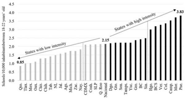
Therefore, this paper analyzes the expansion of the supply of educational spaces at the upper level between 1993 and 2005. This expansive policy was sought to expand educational opportunities in different regions of the country. However, the growth pattern in the number of higher education schools shows important differences in the intensity of the expansion experienced by the different states. Figure 3 illustrates the intensity of the expansion in the different states. The number of new schools built per 10 000 inhabitants between 18 and 22 years between 1993 and 2005 is also shown. As can be seen in figure 2, the national average of new schools built in this period is 2.15 per 10 000 inhabitants of potential age. Some states experienced construction of schools above the national average. For example, Puebla is the state where the expansion of educational spaces during this period occurred with greater intensity; 3.83 new schools were built for every 10 000 inhabitants of potential age. In contrast, some states saw a lower intensity in the construction of educational spaces with respect to the national average. For example, Querétaro is the state that has the lowest intensity of this expansion; only 0.85 new schools were built per 10 000 inhabitants in the potential age range.
In light of this expansion, the construction of schools can be assumed as a treatment with different intensities through two sources of variation. On the one hand, the differences that exist between states where few schools were built against many schools (high vs low intensity). On the other, the differences between the birth cohorts of the people who caused them to be differentially affected by the expansion according to the age threshold at which they were at the time of the expansion. With these considerations, in the following section is explained in more detail the research design that follows the present work.

Note: The number of new schools built per 10 000 inhabitants between 18 and 22 years is shown. Source: Own elaboration with data from the SNIEE population projections presented by the CONAPO in Mexico.
Figure 2 Intensity of the expansion of higher education schools between 1993 and 2005 by states
3. Research design
This section presents in detail the research design used for the empirical analysis.
3.1 Data
This paper uses two sources of information. On the one hand, data from the Module Intergenerational Social Mobility 2016 (Módulo de Movilidad Social Intergeneracional 2016, MMSI-2016) provided by the National Institute of Statistics and Geography (Instituto Nacional de Estadística y Geografía, INEGI) in Mexico. This survey concentrates the attention on the population between 25 and 64 years to capture current and retrospective information (when the respondent was 14 years old) of the socioeconomic and educational characteristics of the informant and his parents, respectively. This generates information that allows comparing the respondents’ current socioeconomic and educational situation against those same characteristics in their origin household. The results derived from the survey are representative at the national level for both the urban area -2 500 or more inhabitantsand the rural one -less than 2 500 inhabitants. This work focuses on a subsample of individuals born between 1961 and 1979. On the other hand, the subsample analyzed in the MMSI-2016 is linked to data from the SNIEE and the number of new higher education schools built between 1993 and 2005 at the state level. This link is determined by identifying the state where the respondent lived when he was 14 years old.
One of the reasons for using the MMSI-2016 is that it allows us to obtain key information for the analysis presented in this paper. Although there are different ways of approaching social mobility, this paper analyzes the effects of the expansion on intergenerational educational and wealth social mobility.10 This implies the need to correlate educational and wealth outcomes between parents and children; by collecting current and retrospective information, the survey allows linking these results. On the one hand, for the analysis of educational mobility, the schooling completed by the respondent and the average years of schooling completed by the respondent’s father and mother are used. On the other hand, two wealth indices are constructed for the analysis of mobility in wealth, one for the current household and another for the respondent’s origin household. These indices are constructed taking the first dimension that resulted from combining a set of goods and services present in the home -current and originthrough a multiple correspondence analysis.11 The inertia of the dimension used for the current household wealth index explains 94.1% of the correlation between goods and services. While the inertia of the origin household wealth index explains it in 96.1%.12
It is worth discussing that the wealth index is constructed from combining a set of goods and services present in the household, which is a measure followed in the literature, particularly to analyze countries where the labor income of both parents and children is not readily available (McKenzie, 2005) as its the case of Mexico. However, despite its widespread use, the interpretation of the construct that captures this index has varied (Torche, 2020). On the one hand, authors indicate that the index empirically approximates household wealth (Filmer and Pritchett, 1999), but, on the other hand, authors tend to interpret it as an index of socioeconomic status or long-term economic situation (McKenzie, 2005; Ferguson et al., 2003; Sahn and Stifel, 2003). In this paper, I interpret the constructed index as an indicator of wealth since combining a series of goods and services in the household represents an effort to mitigate the measurement error that derives from transitory fluctuations in labor income as distinguished by Solon (1992).
3.2 Empirical strategy
The construction of higher-level schools between 1993-2005 can be considered as a treatment with different intensities. In this sense, the exposure of individuals to the expansion of these schools can be identified from two sources of variation: the year of birth and the state where the respondent lived when he was 14 years old. On the one hand, the differences in people’s birth year allow generating two groups differentially affected by the expansion. So, when considering the threshold of potential age at which people attend this educational level, people above that threshold at the time of building schools can be considered as untreated, and people at that threshold or below can be considered as treated. In the particular case of Mexicans, they normally attend higher education between the ages of 18 and 22. All people born in 1971 or earlier were 22 years or older in 1993 when the analyzed educational expansion began. Therefore, they did not benefit from the expansion. For individuals under 22 in 1993, exposure is a growing function of their birth year. Thus, the effect of the program should be close to 0 for individuals 22 years of age or older in 1993 and greater for individuals less than 22 years old. This means that, depending on the birth cohort, there will be individuals who should have been before and after expansion. On the other hand, differences in the intensity of school construction by state (high and low intensity) differentially affected individuals according to the state in which they lived at age 14.
Therefore, constructing a greater number of schools can generate an exogenous variation that induces the potential demand for higher education to accumulate more years of schooling. One way to illustrate this is to imagine a scenario for two individuals. Individual A is 1 year older than individual B. These were born in the same State, the same municipality, the same locality, the same colony, and on the same street. Let us consider identical the observable characteristics of their families, and even similar skills. The difference is that when individual A finished high school, no school offered higher education near his area of influence. For this reason, he concluded his educational career and looked for an option within the labor market. A year later, when individual B finished high school, a higher education school was opened within his area of influence. The opening of that school induced individual B to continue his academic training. In contrast, individual A, who is identical to B except for age, stayed only with the secondary level. It is in this sense that, ceteris paribus, the construction of higher-level schools can represent an exogenous variation in the education of people.
For the empirical analysis, the states are grouped into treated with high and low intensity, following two classifications. First, high intensity states are defined as those that received a school building per 10 000 inhabitants of potential demand above the national average (2.15). While the complement is defined as low intensity states. In this way, the following states are grouped as follows:
High A: Baja California, Baja California Sur, Campeche, Colima, Durango, Guanajuato, Guerrero, Hidalgo, Morelos, Puebla, Sinaloa, Sonora, Tamaulipas, Veracruz, and Yucatán.
Low A: Aguascalientes, Coahuila, Chiapas, Chihuahua, Ciudad de México, Jalisco, Estado de México, Michoacán, Nayarit, Nuevo León, Oaxaca, Querétaro, Quintana Roo, San Luis Potosí, Tabasco, Tlaxcala, and Zacatecas.
Second, as shown in figure 2, there are states that present a construction of schools that are well above and well below the national average. Following figure 2, the states with high intensity are defined from the State of Hidalgo, states where, on average, 3.01 schools were built per 10 000 inhabitants of potential demand, which is well above the national average (2.15). While the low intensity states were defined from the state of Nayarit, where, on average, 1.84 schools were built for every 1 000 inhabitants of potential demand, which is well below the national average (2.15). In this way the following states are grouped as follows:
High B: Baja California Sur, Campeche, Colima, Hidalgo, Morelos, Puebla, and Veracruz.
Low B: Aguascalientes, Chiapas, Chihuahua, Jalisco, Estado de México, Michoacán, Nayarit, Nuevo León, Oaxaca, Querétaro, Tabasco, Tlaxcala, and Zacatecas.
Table 2 presents some descriptive statistics of interest. There are 12 960 individuals in the subsample analyzed with an average level of schooling of 9.33 degrees of education completed. This represents little more than the finished middle school. On average, 2.15 new schools were built per 10 000 inhabitants between 18 and 22 years during the period of expansion analyzed (1993-2005). For states that experienced a high intensity of expansion (High A), an average of 2.82 new schools were built per 10 000 individuals of potential age. For low intensity states (Low A), 1.56 new schools were built per 10 000 inhabitants aged 18-22. Likewise, for states that experienced a high intensity of expansion (High B), an average of 3.42 new schools were built per 10 000 individuals of potential age. In the case of low intensity states (Low B), 1.38 new schools were built per 10 000 inhabitants aged 18-22.
Table 2 Descriptive statistics
| Variable | Mean | Est. dev. |
| Average schooling (whole sample N = 25 363) | 9.62 | 4.5521 |
| Average schooling (sub-sample N = 12 960) | 9.33 | 4.494 |
| (cohort born between 1961 and 1979) | ||
| New schools built per 10 000 individuals between 18-22 years old (1993-2005) | 2.15 | 0.8207 |
| (High A) States with high intensity. New schools built per 10 000 individuals between 18-22 years old (1993-2005) | 2.82 | 0.6138 |
| (Low A) States with low intensity. New schools built per 10 000 individuals between 18-22 years old. (1993-2005) | 1.56 | 0.4254 |
| (High B) States with high intensity. New schools built per 10 000 individuals between 18-22 years old (1993-2005) | 3.42 | (0.2714) |
| (Low B) States with low intensity. New schools built per 10 000 individuals between 18-22 years old. (1993-2005) | 1.38 | (0.2987) |
Source: Own elaboration with data from MMSI-2016 and the SNIEE.
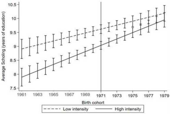
Figure 3 compares the change in the average level of schooling of individuals in both groups classified as the treated group (lived in a high intensity entity and were at the age threshold for higher education) and the group defined in this paper as untreated (lived in a low intensity entity and were at the age threshold where they are assumed to be less willing to pursue higher education even if a new school is built). As can be seen, in both groups there was an increase in schooling, however, the group defined as treated show a faster increase starting at the threshold age considered to be treated, that is, those who were born in 1971 (who were 22 years old in 1993, the year in which the expansion analyzed began). However, in the case of both groups, treated and untreated, parallel trends can be seen in birth cohorts before 1971.
The effects of this differential treatment can be shown in a table of mean differences. Table 3 shows the education averages for different cohorts and intensities of school construction. For this comparison is used the states grouped into “High A and “Low A” that was defined previously. Thus, the educational achievement of the group of people who had little or no exposure to the program (they were between 22 and 26 years old in 1993) is compared with those of the people who were exposed to the expansion (they were between 14 and 18 years old in 1993) for both groups of states. As can be seen, in both groups of states compared, the average schooling increased over time. However, it increased more in the states where more schools were built. The difference in this difference can be interpreted as the causal effect of educational expansion under the assumption that, in the absence of expansion, the increase in average schooling would not have been systematically different in high and low intensity states. An individual at the age threshold to be affected by the expansion and born in state with high intensity of school construction received, on average, 0.582 years more education.
Table 3 Average schooling for treated and untreated cohorts by intensity of treatment
| Average schooling (years of education) | |||
| School construction intensity | |||
| Cohorts | High A | Low A | Difference |
| Experiment of interest | |||
| 14-18 years old in 1993 | 9.77 | 9.947 | -0.177 |
| (0.1303) | (0.1412) | (0.1921) | |
| 22-26 years old in 1993 | 8.805 | 9.564 | -0.759 |
| (0.14) | (0.1588) | (0.2117) | |
| Difference | 0.965 | 0.383 | 0.582 |
| (0.1913) | (0.2125) | (0.2859) | |
| Control experiment | |||
| 22-26 years old in 1993 | 8.805 | 9.564 | -0.759 |
| (0.14) | (0.1588) | (0.2117) | |
| 27-32 years old in 1993 | 8.193 | 9.041 | -0.848 |
| (0.1547) | (0.1658) | (0.2268) | |
| Difference | 0.612 | 0.523 | 0.089 |
| (0.2087) | (0.2296) | (0.3112) | |
| Subsample (1961-1979) | 9.33 | ||
| N=12 960 | (0.0394) | ||
| General (1952-1991) | 9.62 | ||
| N=25 363 | (0.0285) | ||
Note: Robust standard errors in parentheses. States that received school construction above the national average (2.15) are grouped “High A”, while complement is grouped as “Low A”.
Source: Own elaboration.
Given the assumption of parallel trends, this result depends on the assumption that, in the absence of expansion, the increase in schooling among individuals whose age threshold was large enough not to be affected by the expansion, should not systematically vary between high and low intensity states. Table 3 attempts to prove this with a control experiment. For this, two cohorts are considered at an age threshold large enough not to be affected for expansion; individuals between 22 and 26 years old in 1993 and individuals between 27 and 32 years old in 1993. The difference in difference estimated of these cohorts and different intensities of the expansion is 0.089, which is very close to 0 and is not statistically significant. These results provide some suggestive evidence that the differences in differences are not driven by inappropriate identification assumptions, although they are imprecisely estimated.
Similarly, table 4 concentrates the intergenerational correlation of education and wealth for the different cohorts and intensities of school building at the higher level. As can be seen, the estimated results for educational mobility show that, in both cohorts, intergenerational educational persistence declined over time. However, there was a slightly greater decrease in the states that experienced a high intensity of expansion. The difference in difference is -0.024, however, this is not statistically significant. In the case of mobility in wealth, it is observed that, in both cohorts, the intergenerational persistence of wealth increased slightly over time. However, it increased slightly more in the case of low intensity states, although the difference in difference is not statistically significant. In the following subsection this strategy is developed based on the regression analysis that allows different control variables to be included to obtain more convincing results.
Table 4 Intergenerational correlation of wealth and education for treated and untreated cohorts by intensity of treatment
|
Intergenerationall correlation of education* |
Intergenerationa correlation of wealth** |
|||||
| Intensity | Intensity | |||||
| High A | Low A | Diff | High A | Low A | Diff | |
| Experiment of interest | ||||||
| 14-18 years old in 1993 | 0.588 | 0.636 | -0.048 | 0.645 | 0.729 | -0.084 |
| (0.025) | (0.021) | (0.033) | (0.024) | (0.026) | (0.036) | |
| 22-26 years old in 1993 | 0.643 | 0.667 | -0.023 | 0.628 | 0.709 | -0.081 |
| (0.035) | (0.034) | (0.049) | (0.027) | (0.028) | (0.039) | |
| Difference | -0.055 | -0.031 | -0.025 | 0.017 | 0.02 | -0.003 |
| (0.044) | (0.04) | (0.059) | (0.037) | (0.038) | (0.053) | |
| Control experiment | ||||||
| 22-26 years old in 1993 | 0.643 | 0.667 | -0.024 | 0.628 | 0.709 | -0.081 |
| (0.035) | (0.034) | (0.049) | (0.027) | (0.028) | (0.039) | |
| 27-32 years old in 1993 | 0.757 | 0.788 | -0.031 | 0.662 | 0.68 | -0.018 |
| (0.051) | (0.03) | (0.059) | (0.025) | (0.029) | (0.039) | |
| Difference | -0.114 | -0.121 | 0.007 | -0.034 | 0.029 | -0.063 |
| (0.062) | (0.046) | (0.077) | (0.037) | (0.04) | (0.055) | |
| Subsample (1961-1979) | 0.66 | 0.62 | ||||
| (0.0084) | (0.01) | |||||
| N | 12 734 | 12 649 | ||||
| General (1952-1991) | 0.64 | 0.60 | ||||
| (0.0053) | (0.0073) | |||||
| N | 24 908 | 24 851 | ||||
Notes: *The mean schooling of the father and mother is correlated with the schooling of the child. **The index of wealth of the home of origin is correlated with the index of wealth of the current household, both variables have been standardized with zero mean and standard deviation of 1. Robust standard errors in parentheses. States that received school construction above the national average (2.15) are grouped “High A”, while complement are grouped as “Low A”.
Source: Own elaboration.
4. Results
The following subsections account for the estimated empirical results in four directions. First, the results of the effect of the expansion on the average schooling of individuals are estimated. Second, the effect of educational expansion on educational intergenerational social mobility is estimated. Third, the estimated results of the effect of expansion on the intergenerational social mobility of wealth are presented. Finally, an analysis is presented on the redistribution of the new educational opportunities created between the different socioeconomic strata.
4.1 Effects on schooling
This section seeks to assess whether the construction of new educational spaces led to gains in the education of individuals. For this, the following econometric specification is estimated:
where S ist captures the education of the individual i who lived in the state s at age 14, and was born in year t. c 1 is the constant of regression. ∝ s is a state dummy variable and capture fixed effects of the state where the individual lived at age 14. β t absorbs fixed effects of the birth cohort. H s is a dummy that indicates high intensity of the construction of schools in the state s. T i is a dummy that indicates whether the individual belongs to the cohort treated in the subsample (1 = 14-18 years in 1993, 0 = 22-26 years in 1993). Z s is a vector of control variables that capture specific characteristics of states. They include: real growth rate of GDP per capita between 1994 and 1995; net rate of non-enrollment in higher education in 1992;13net enrollment rate for primary, secondary and upper secondary education levels in 1992.14 Finally, ε ist is the error term. The parameter γ 1 is the one of interest and accounts for the coefficient of differences in differences.
Table 5 presents the estimated results for equation (1). The results compare the average schooling of individuals between 14-18 years old in 1993 (treated cohort) and individuals between 22-26 years old in 1993 (control cohort). Column 1 is the simple specification, that is, without control variables. The estimated coefficient is statistically significant with a 90% level of confidence and suggests that a new higher education school built per 10 000 individuals potential age to attend higher education (18-22 years) led to an average increase of 0.52 more years of education of the treated cohort. However, this interpretation is based on the identification assumption that there are no omitted effects that vary over time or specific characteristics of each state that can potentially be correlated with expansion. For example, the expansion of schools may be associated with the potential demand for higher education in each state. The identification assumption will also be violated if macro factors such as the macroeconomic situation (GDP) are correlated with the expansion of schools.
Table 5 Estimated results: effect of the construction of higher education schools on average schooling
| Average Schooling (years of education) | ||||
| Variables | High and Low A | High and Low B | ||
| (1) | (2) | (3) | (4) | |
| High intensity ## treated cohort | 0.52* | 0.60** | 0.90** | 1.027*** |
| (0.277) | (0.293) | (0.398) | (0.4112) | |
| Control variables | ||||
| GDP growth rate 94-95 ## treated cohort | No | Yes | No | Yes |
| Higher non-enrollment rate 92 ## treated cohort | No | Yes | No | Yes |
| Upper secondary net enrollment rate 92 ## treated cohort | No | Yes | No | Yes |
| Secondary net enrollment rate 92 ## treated cohort | No | Yes | No | Yes |
| Primary net enrollment rate 92 ## treated cohort | No | Yes | No | Yes |
| N | 7 188 | 7 188 | 4 461 | 4 461 |
| R2 | 0.074 | 0.076 | 0.059 | 0.061 |
Notes: Only the interest coefficient of equation (1), γ1, is reported. All regressions include states dummies where the respondent lived at age 14 and birth cohort dummies. Robust standard errors in parentheses. Level of statistical significance: ***p<0.01, **p<0.05, *p<0.1.
Source: Own elaboration.
For above, column 2 presents the results of regressions that control the specific characteristics of the states and their interaction with the treated cohort. Control variables included are: the real growth rate of GDP per capita between 1994 and 1995, the net non-enrollment rate for higher education in 1992, and the net enrollment rate for the primary, secondary and upper secondary education level in 1992. The estimated results show an underestimation of the causal effect in the initial regression. The effect of expansion after controlling for statespecific characteristics and their interaction with the treated cohort suggests with the 95% level of confidence that a new higher education school built per 10 000 individuals of potential age to attend higher education (18-22 years), led to an average increase of 0.60 more years of education for individuals at the age threshold affected by the expansion and born in a state with high school construction intensity received, in this paper considered as the treated cohort.
Columns 3 and 4 show the simple estimation and with control variables, respectively, when comparing the states with greater and lesser intensity in the construction of schools. As you can see, although the estimated coefficients are larger, they are consistent with the previous ones. In this sense, the results allow us to determine that the educational policy that seeks to expand the supply of schools at a higher level can induce the population to accumulate more years of schooling. However, how did the construction of new schools affect the structure of opportunities for social mobility? The following subsections examine this question.
4.2 Effects on educational intergenerational social mobility
This section quantifies the effect of the construction of new educational spaces at the higher level on educational intergenerational social mobility. This refers to the intergenerational correlation of educational results between parents and children. This effect is identified from estimating the following econometric specification:
Where
Table 6 gives an account of the estimated results for equation (2). Column 1 presents the results when control variables are not included. The results with this specification show, on the one hand, the educational intergenerational correlation of the order of 0.62. This result has a 99% level of confidence. On the other hand, the estimated effect of the expansion of higher education on educational mobility, although it follows the expected (negative) sign, is not a statistically significant effect. Column 2 reports the results by controlling for the specific characteristics of the states and their interaction with the treated cohort. The control variables included are: the real growth rate of GDP per capita between 1994 and 1995, the net non-enrollment rate for higher education in 1992, and the net enrollment rate for primary, secondary and upper secondary education level in 1992. The results suggest no statistically significant effect between the construction of new higher education schools and educational social mobility.
Columns 3 and 4 show the simple estimation and with control variables, respectively, when comparing the states with greater and lesser intensity in school construction. The results are consistent with the previous ones: I found no statistically significant effect between the expansion of schools at the higher level and educational social mobility.
Table 6 Estimated results: effect of the construction of higher education schools on educational intergenerational social mobility
| Children’s schooling (years of education) | ||||
| Variables | High and Low A | High and Low B | ||
| (1) | (2) | (3) | (4) | |
| Parents’ schooling | 0.62*** | 0.61*** | 0.63*** | 0.63*** |
| (0.034) | (0.035) | (0.339) | (0.04) | |
| Parents’ schooling ## intensity | -0.031 | -0.045 | -0.019 | -0.018 |
| high ## treated cohort | (0.0586) | (0.0592) | (0.087) | (0.087) |
| Control variables | ||||
| GDP growth rate 94-95 ## treated cohort | No | Yes | No | Yes |
| Higher non-enrollment rate 92 ## treated cohort | No | Yes | No | Yes |
| Upper secondary net enrollment rate 92 ## treated cohort | No | Yes | No | Yes |
| Secondary net enrollment rate 92 ## treated cohort | No | Yes | No | Yes |
| Primary net enrollment rate 92 ## treated cohort | No | Yes | No | Yes |
| N | 7 071 | 7 071 | 4 395 | 5 48 |
| R2 | 0.348 | 0.35 | 0.349 | 0.351 |
Notes: Only the interest coefficient of equation (2), γ4, is reported. All regressions include states dummies where the respondent lived at age 14 and birth cohort dummies. Robust standard errors in parentheses. Level of statistical significance: ***p<0.01, **p<0.05, *p<0.1.
Source: Own elaboration.
4.3 Effects on intergenerational social mobility of wealth
In this section the effect of the construction of new educational spaces at the higher level on the intergenerational social mobility of wealth is quantified. This refers to the intergenerational correlation of socioeconomic outcomes between parents and children. This effect is identified from estimating the following econometric specification:
where
Table 7 presents the estimated results for equation (3). Column 1 shows the results when control variables are not included. The first result that jumps immediately, with a 99% level of confidence, is the intergenerational correlation of wealth of the order of 0.64. This means that increasing the wealth of the household of origin by one standard deviation is associated with an increase of 0.64 standard deviations in the wealth of the current household. On the other hand, it can be seen that the estimated effect of the expansion of higher education on the intergenerational social mobility of wealth is not statistically significant. Column 2 reports the results by controlling for the specific characteristics of the states and their interaction with the treated cohort. Similarly, the results suggest no statistically significant effect between the construction of new higher education schools and the intergenerational social mobility of wealth.
Table 7 Estimated results: effect of the construction of higher education schools on the intergenerational social mobility of wealth
| Children’s wealth | ||||
| Variables | High and Low A | High and Low B | ||
| (1) | (2) | (3) | (4) | |
| Parents’ wealth | 0.652*** | 0.64*** | 0.66*** | 0.66*** |
| (0.03) | (0.0315) | (0.033) | (0.034) | |
| Parents’ wealth ## intensity high | 0.001 | -0.008 | 0.044 | 0.042 |
| ## treated cohort | (0.0534) | (0.0558) | (0.078) | (0.08) |
| Control variables | ||||
| GDP growth rate 94-95 ## treated cohort | No | Yes | No | Yes |
| Higher non-enrollment rate92 ## treated cohort | No | Yes | No | Yes |
| Control variables | ||||
| Upper secondary net enrollment rate 92 ## treated cohort | No | Yes | No | Yes |
| Secondary net enrollment rate 92 ## treated cohort | No | Yes | No | Yes |
| Primary net enrollment rate 92 ## treated cohort | No | Yes | No | Yes |
| N | 6 949 | 6 949 | 4 319 | 4 319 |
| R2 | 0.416 | 0.4179 | 0.43 | 0.43 |
Notes: Only the interest coefficient of equation (2), γ4, is reported. All regressions include states dummies where the respondent lived at age 14 and birth cohort dummies. Robust standard errors in parentheses. Level of statistical significance: ***p<0.01, **p<0.05, *p<0.1.
Source: Own elaboration.
Columns 3 and 4 show the simple estimation and with control variables, respectively, when comparing the states with greater and lesser intensity in school construction. The results are consistent with the previous ones: I found no statistically significant effect between the expansion of schools at the higher level and the intergenerational social mobility of wealth.
The previous findings show that educational expansion through offering a greater number of higher education schools leads to gains in people’s schooling, but does not necessarily promote social mobility. As discussed in the literature review, promoting social mobility will depend on how new educational opportunities are distributed among different socioeconomic strata (Marginson, 2016). The following subsection examines to what extent the educational policy of expansion of schools at the higher level has managed to provide more equitable access to higher education for Mexicans (i.e., who benefited the expansion?).
4.4 Who benefited the expansion?
As stated above, the possibility of creating equal opportunities through constructing new educational spaces depends on how the new educational opportunities are distributed among individuals from different socioeconomic strata. This section explores the changes in time in the achievement of higher education (more than 12 years of scholing) among individuals from different socioeconomic strata according to the exposure or not they had during the construction of new spaces of higher education. As stated before, the birth cohort and the state where the respondent lived at age 14 allow two groups to be differentially affected by the construction of higher-level schools. To account for this, the following logistic regression model is estimated:
Where higher_education = 1 is a dummy that indicates whether the individual i who lived in the state s at age 14, and was born in year t, has more than 12 years of schooling. ∝
s
is a state dummy variable and capture fixed effects of the state where the individual lived at age 14. β
t
absorbs fixed effects of the birth cohort.
Based on the estimated results of the previous model, the predicted probabilities for the two groups of individuals differentially affected by the expansion are extracted. Figure 4 shows the predicted probabilities of obtaining higher education (more than 12 years of schooling) conditional on the wealth quintile of the household of origin for these groups. When comparing the results of both groups (treated and untreated) it can be seen that the probability of reaching higher education for treated individuals increased for the richest wealth quintiles (III, IV and V). While that this probability decreased slightly for the poorest wealth quintiles (I and II).
Notes: Probabilities predicted by the logistic model estimated in equation (4). The probability of reaching higher education (more than 12 years of schooling) for the two groups of individuals differentially affected by the expansion according to their birth cohort and the state where they lived at age 14 is illustrated. 4,319 observations. Source: Own elaboration with data from MMSI-2016 and SNIEE.
Figure 4 Predictive margins with 95% cis
These results suggest that the distribution of the new educational opportunities created occurred unequally among the different socioeconomic strata. With this, those who ended up benefiting from the construction of new higher education schools were people whose households of origin had a greater socioeconomic advantage. Specifically, the probability of reaching higher education for individuals from the richest quintile and not exposed to the expansion was 49.4%, while individuals from that same quintile but who were exposed to the expansion have a probability of 63.3% of reaching this educational level. In contrast, individuals whose home of origin belongs to the poorest wealth quintile and not exposed to expansion, have a probability of reaching higher education of 3.1%, while individuals from that same quintile but who were exposed to expansion have a 1.9% chance of reaching that educational level. These results suggest that the expansion of higher education disproportionately benefited individuals from relatively wealthy families. As a result, the inequality of educational opportunities faced by the extremes of socioeconomic distribution increased.
5. Conclusions
The private return that higher education offers places it as a potential route that increases the probabilities of a rise in the socioeconomic structure. As a result, one of the axes of education policy in many governments has been oriented to expand this educational level by increasing the supply of higher education schools. However, the scope of this type of policy in the creation of equal opportunities is not clear since it depends largely on how new educational opportunities are distributed among the different socioeconomic strata. This paper analyzed the potential contribution of the expansion of schools at the higher education over the level of schooling and intergenerational social mobility in Mexico. For this, a data set was used that links the results of 2016 Mexican Social Mobility survey with information from the National System of Educational Information on the construction of schools at tertiary education that occurred between 1993 and 2005 at the level of states. The expansion of the supply of educational spaces serves as a natural experiment that allows the variation in the construction of schools to be exploited through birth cohorts and the state where the respondent lived at the age of 14.
It is worth highlighting some limits and scope of this work. On the one hand, it is necessary to clarify the scope of the causality identified. The strategy allows producing causal estimates of the construction of higher-level schools on individuals’ educational achievement. But the causality identified in relating this expansion of schools with the intergenerational social mobility of education and wealth is more difficult. This is so for the following reason: the growth of the offer of educational spaces at the upper level, for the case of Mexico, took place gradually and was not an abrupt change due to some specific reform. In this sense, both expansion and educational and wealth outcomes may likely be affected by supply and demand factors. However, the paper tries to correct this limitation by including a series of variables that allow controlling most of the spatial and temporal heterogeneity between the states. Moreover, there is a variable that, due to data restrictions, has been left out of this analysis. This refers to the quality of the schools that are built. The literature shows that the quality of the new schools built is key to explaining the success of a policy that seeks to redistribute educational opportunities for intergenerational social mobility (Brezis and Hellier, 2018; Liu and Wan, 2017; Lucas, 2001). Unfortunately, the data used here does not allow us to capture approximations for these variables.
Another limitation to consider is that, given the restriction of the information available to me, it is not possible to quantify educational expansion at a lower level of disaggregation than that of states, such as municipalities or localities. This is important to consider, as this paper assumes that the presence of new schools in the state regardless of the remoteness of a given locality from the school is relevant to households’ decision to send their children to school. Unfortunately, I do not have information available to show whether the construction of these educational spaces was concentrated in large cities or urban areas as compared to rural areas. For this reason, the results found and discussed should be taken with caution.
The findings regarding the effects of educational expansion on schooling suggest that the availability of a greater number of higher education schools led to gains in the schooling of individuals affected by these school’s construction. The estimated effect is statistically significant with a 95% level of confidence. It suggests that a new school of higher education built per 10 000 individuals on potential age (between 18 and 22 years) increased the average schooling of the treated cohort (they were between 14 and 18 years in 1993) in 0.60 years more years of education. On the other hand, when analyzing the results of the expansion on educational intergenerational social mobility, it was found that, with a 99% level of confidence, the intergenerational educational persistence of the order of 0.62 is confirmed. However, by linking the expansion of higher-level schools and their effect on educational mobility, no statistically significant evidence was found. Likewise, the results found regarding the intergenerational social mobility of wealth show, on the one hand, an intergenerational correlation of the current and origin socioeconomic conditions of the order of 0.64 with 99% level of confidence. On the other hand, no statistically significant evidence was found that the expansion of higher education modified this structure of opportunities.
In addition, it was explored how the new educational opportunities created among the different socioeconomic strata were distributed. When comparing the results of groups differentially affected by the expansion, it was found that the probability of reaching higher education for treated individuals increased for the richest wealth quintiles (III, IV, and V). While that this probability decreased slightly for the poorest wealth quintiles (I and II). Specifically, the probability of reaching higher education for individuals from the richest quintile and not exposed to the expansion was 49.4%, while individuals from that same quintile but who were exposed to the expansion have a probability of 63.3% of reaching this educational level. In contrast, individuals whose home of origin belongs to the poorest wealth quintile and were not exposed to expansion have a probability of reaching higher education of 3.1%, while individuals from that same quintile but who were exposed to expansion have a 1.9% chance of reaching that educational level. These results suggest that the expansion of higher education disproportionately benefited individuals from relatively wealthy families. As a result, the inequality of educational opportunities faced by the extremes of socioeconomic distribution increased.
These findings suggest that, despite the State’s effort to expand the supply of educational facilities at the higher level, inequities in access continue to be maintained. Although on average, there have been gains in the schooling of the population, the truth is that the distribution of the new educational opportunities created has occurred unequally among the different socioeconomic strata. With this, those who ended up benefiting from the construction of new higher education schools were people whose households of origin had a greater socioeconomic advantage. This translates into the fact that the population with the greatest socioeconomic disadvantage continues to be excluded from higher education. Consequently, intergenerational social mobility patterns can be reproduced. In this sense, it is important to recognize that the expansion of higher education through the distribution of new educational spaces will not promote intergenerational social mobility on its own. It is also necessary to implement parallel efforts to strengthen the quality of schools, the market employment and equal opportunities in other aspects. This raises the need to redirect educational policies to set aside the concern of how many people arrive and complete the university. Instead, the concern should focus on who arrives and completes this educational level. For example, the expansion of schools should be more sensitive to the barriers faced by historically excluded people such as women, indigenous people and the poorest population.
Finally, education alone is not the only force that must be fostered to promote intergenerational social mobility. A synchronized effort of a set of policies is required to address this problem. For example, the necessary dialogue between education and the labor market is an issue that should be prioritized to improve equal opportunities. Also, fiscal policy and redistribution through public spending point in the same direction.

