


Services on Demand
Journal
Article
 text in
  English (pdf)
 Article in xml format
 Article references
 Send this article by e-mail
Indicators
-
 Cited by SciELO
 -
 Access statistics
Related links
-
 Similars in
SciELO
Similars in
SciELO
Share

 Permalink
Contaduría y administración
Print version ISSN 0186-1042
Contad. Adm vol.67 n.3 Ciudad de México Jul./Sep. 2022 Epub June 06, 2023
https://doi.org/10.22201/fca.24488410e.2022.3290
Articles
Longevity-risk hedge with derivatives: Mortality estimation and simulations with data from Mexico
1Universidad Autónoma de Guadalajara, México
2 Instituto Tecnológico y de Estudios Superiores de Occidente, México
3Universidad de Guadalajara, México
The objective of this article is to show the feasibility of derivative products being used to hedge longevity risk in Latin America. To do this, a longevity index is built with Mexican data using the Lee-Carter model and several longevity-linked derivatives are simulated. Results indicate that an ecosystem of derivative instruments is feasible in Mexico for two reasons: they are effective as hedging against longevity risk and the estimated longevity index, used as an underlying asset, does not correlate with relevant stock indices, which makes it feasible as part of a comprehensive financial portfolio. The originality of this research consists in the adaptation for Mexico of novel valuation methodologies and the new estimation of a longevity index. The main limitation of this research is that the ecosystem is subject to a base risk with respect to the population structure in the future
JEL Code: G22; G23; H55; J11; J26
Keywords: longevity; options; pensions; swaps; swaptions
El objetivo de este artículo es mostrar la factibilidad de que productos derivados sean utilizados como cobertura del riesgo de longevidad en Latinoamérica. Para ello, se construye un índice de longevidad con datos mexicanos usando el modelo Lee-Carter y se simulan diversos instrumentos derivados de longevidad. Se concluye que un ecosistema de instrumentos derivados es factible en México por dos razones, éstos son efectivos como cobertura del riesgo de longevidad y el índice de longevidad construido, y utilizado como activo subyacente, no presenta correlación con índices accionarios relevantes, lo que lo hace factible como parte de un portafolio financiero amplio. La originalidad de este trabajo consiste en la adaptación de metodologías de valuación inéditas para México y la estimación de un índice de longevidad propio, y la principal limitante es que el ecosistema está sujeto a un riesgo base con respecto a la estructura poblacional en el futuro.
Código JEL: G22; G23; H55; J11; J26
Palabras clave: longevidad; opciones; pensiones; swaps; swaptions
Introduction
Longevity risk, defined as the possibility of living longer than estimated, plays an important role in retirement. An unexpected increase in the years of life in a generation implies that the period in which workers will receive a retirement pension will be extended in the case of a defined benefit scheme or that the pensioner will have an insufficient scheduled retirement plan in the last years of life or potential insolvency in the case of a life annuity in a defined contribution scheme. These effects are negative for the financial equilibrium of the organizations and individuals bearing the longevity risk, be it a government, a pension institution, or a pensioner.
In practice, the financial effects of longevity risk have been handled differently. Some institutions or individuals accept the risk in exchange for some compensation or premium, others use insurance or reinsurance to spread the likely losses, and some institutions turn to financial markets using derivative instruments to manage this risk (Blake, 2018). To a certain extent, the latter alternative has been used more in recent years because the longevity market is attractive to investors because it offers assets that are not correlated with other financial assets (Jamal & Quayes, 2004), thus providing opportunities to diversify investment portfolios and create more efficient strategies.
The first public longevity swap contract was between Swiss Re and Provident in 2007, worth approximately £1.7 billion, with Swiss Re paying observed mortality to Provident in exchange for a preset premium. In 2008 a swap was completed with Canada Life hedging £500 million of its annuity plan through a 40-year contract. In this case, the longevity risk was transferred to insurance-linked asset (ILS) investors and hedge funds. Credit Suisse subsequently entered a survival swap in 2009 to hedge the longevity risk of the Babcock International pension plan in the United Kingdom. In terms of non-linear derivatives, in 2012 and 2013, Aegon negotiated hedges with Deutsche Bank and Société Générale. Also, in 2014 and 2015, Delta Lloyd and Reinsurance Group of America were involved in transactions of this nature. By 2018, the size of the global longevity market was estimated to be between $60 billion and $80 billion (Blake, 2018).
This series of successes has not been replicated in Latin American financial markets, where no successful issuance of this type of instrument has yet been reported, despite theoretical developments applied to Mexico in longevity swaps (Rodríguez, 2017) and longevity bonds (Cruz et al., 2018), and the attempt to issue a longevity bond promoted by the World Bank and the Chilean Superintendency of Securities and Insurance in 2010, which ultimately did not materialize (Blake et al., 2013).
This article aims to show the feasibility of longevity risk management through long- and short-term longevity financial derivatives in Latin American countries, attractive to local and global investors as assets not correlated with other financial assets, to promote their adoption in Latin America. Mexico is used as an example in the estimations, using the longevity swap proposal of Rodriguez (2017) as a starting point.
To show feasibility, first it is necessary to structure a longevity index that offers a speculative and diversification element for investors unrelated to the pension sector and develop forecasts of life expectancy in Mexico with the Lee and Carter (1992) model. Second, a long-term longevity swap for Mexico is structured like the one proposed by Rodriguez (2017) but based on the new longevity index. Third, based on the methodology of Cairns et al. (2010), a series of derivatives based on the longevity index proposed in this article were valued, showing that these instruments can be used to carry out hedging strategies that transfer the longevity risk of a pension system to different interested participants. This indicates that these instruments can reduce longevity-related uncertainty and create opportunities for hedging and portfolio diversification.
The following section addresses the literature review, followed by estimating a mortality index for Mexico using the methodology of Lee and Carter (1992). Then there is a section that structures and simulates the longevity derivatives proposed by Cairns et al. (2010) and Rodriguez (2017) with data from Mexico. The main results of this research are presented and finally the conclusions are presented.
Literature review
The literature on the longevity of financial derivative instruments has been growing in recent years. Several authors have contributed to the subject since the beginning of the 21st century, developing financial instruments of greater complexity for managing longevity risk as an integrated body of knowledge has been built up. For example, in the work of Blake and Burrows (2001), the idea of dealing with mortality uncertainty through bonds emerges. In their paper, they argue that the government can issue these instruments, whose coupons depend on the percentage of people who survive each period, starting from an initial group. Subsequently, Cox and Lin (2004) propose the use of longevity swaps as a protection against the risk incurred by companies that offer two lines of insurance: life insurance and annuities. Since they are exposed to mortality from both perspectives and with opposite effects in each line, it is feasible for them to enter a contract of this type within the same company. However, their methodology implies the development of at least two longevity indices for each contract, which can make it difficult to apply in practice (Rodriguez, 2017). A next step in the methodological development of this type of instrument is provided by Dowd et al. (2006). They calculate the value of a swap with a mortality index as the underlying value, which decreases as the members of the closed group with which it is calculated die. The authors seek to give consistency to the price by incorporating the payment of a premium into the fixed part of the swap to equalize the present value of the flows expected for this and the floating part at the beginning of the contract.
Another important element in the literature is provided by Dawson et al. (2009). After the success of derivatives with linear payoffs, such as forwards and swaps, they mention that option-based contracts are the next step in consolidating derivatives markets. Using the premium developed by Dowd et al. (2006), they propose a way to value options with a normally distributed underlying value and apply it to the swap premium after demonstrating that it follows approximately that probability distribution. Likewise, they implement their methodology in a longevity swaption, this type of contract being an option on the swap described in their work. It is important to note that this valuation proposal is employed later in this research. Finally, Cairns et al. (2010) synthesize the valuation methodologies of forwards, swaps, and some types of mortality-based options, thus compiling the findings in the valuation of longevity derivatives into a consistent analytical body, some of which are used in this research.
Concerning Mexico, Rodriguez (2017) mentions that with the 1997 social security reform, the burden of the longevity risk of future generations was transferred from the Mexican government to annuity providers in exchange for a premium partially financed by pensioners' retirement savings. However, this reform made possible a long transition period in which the pay-as-you-go generation maintained their rights and their associated longevity risk was left to the Mexican government. Tapen (2012) estimates that without further changes in pension systems, the fiscal costs of the pay-as-you-go generation will reach a cumulative deficit of about 6% of GDP by the mid-2030s. Likewise, Alonso et al. (2015) project that the fiscal cost of pension obligations of the Mexican Social Security Institute (IMSS) will peak in 2045 when it totals 1.4% of the 2012 GDP.
In this context and with the possibility that these scenarios are underestimated due to potential improvements in longevity, Rodriguez (2017) proposes a long-term longevity swap between the Mexican government and a consortium of life insurance and reinsurance companies as counterparties. For the modeling, said author uses the methodology of Dowd et al. (2006) as a basis, proposing two adaptations to make the model consistent with the reality of the pension systems of Mexico and other Latin American countries. The first is a proportional longevity index that allows for contracts in open groups of pensioners, i.e., in groups that pensioners may enter through the acquisition of rights and not only leave due to mortality, since previous models only considered the latter in their structuring. Secondly, the author establishes a monetization function to reflect the particularities of pension updating in the old Mexican pay-as-you-go (PAYG) system, which applies to pensioners of the previous generation who contributed prior to the 1997 reform.
This article takes Rodriguez (2017) as a basis, and significant modifications are made to the methodology. For example, a different longevity index is constructed and used to make it more attractive to investors. The modified methodology proposed in this article uses period life expectancy since this type of measurement has no direct influence on the prices of financial assets (Denuit, 2009). Therefore, a life expectancy index is constructed using the Lee and Carter (1992) methodology. Subsequently, a longevity swap is constructed and simulated with a structure like that of Rodriguez (2017) with the new longevity index and an ecosystem of derivatives such as forwards, cap options, and swaptions, representing a good alternative to the swap given the greater flexibility and liquidity they provide to the longevity market (Dowd et al., 2006). The use of options provides a considerable range of strategies for interested parties, facilitating the distribution of the risk incurred by inserting other market participants from outside the pension sector.
In addition to the theoretical framework presented, which proposes the management of longevity risk through derivative instruments and has shown feasibility in financial markets in developed countries, several recent studies analyze other schemes to address longevity risk. For example, D'Amato et al. (2018) propose a longevity buy-in strategy that aims to reduce long-term longevity risk for a pension provider under the assumption of a closed group of pensioners and a defined contribution scheme. In this type of contract, the pension provider transfers a longevity risk limited to the difference between two life scenarios (base and pessimistic), considering a specific age range. In exchange for this coverage, the pension provider pays an upfront premium to its counterparty. It is important to mention that this type of coverage leaves out longevity events worse than the pessimistic scenario determined ex-ante.
Another alternative for managing longevity risk is analyzed by Berstein and Morales (2021) with a study on universal longevity insurance in a defined contribution scheme such as the Chilean one. For this purpose, they analyze an increase in the contribution rate throughout the worker's life to fund insurance covering a pension at an advanced age. People who opt for programmed retirement would benefit from a minimum income pension from the age at which the longevity insurance comes into effect, independent of the pension they receive today. Those who opt for a life annuity receive a pension higher than the current scheme.
Broeders et al. (2021) analyze the possibility of sharing longevity risk, at the macro level, among different generational cohorts, based on the premise that this risk affects them differently. If a fixed retirement age is considered, the gain from generational sharing of longevity risk is marginal, from 0.1% to 0.3% in terms of post-retirement consumption equivalents. If the scenario of a flexible retirement age dependent on life expectancy is analyzed, the gains of the scheme improve (from 1.8% to 2.9%). This occurs because the labor supply of active workers acts as a hedge against longevity risk.
Finally, Balter et al. (2021) study the choice between two types of financial products available in the Danish pension system. The first option presented to Danish pensioners is a product with low risk and return but which protects against longevity risk. The second option is a financial product offering higher risk and expected return but higher longevity risk. In the absence of improvements in life expectancy, the product with higher return dominates the product with higher longevity coverage; however, the same is not true in the case of improvements in life expectancy, despite the higher financial gains of the riskier product. The authors conclude that the combination of financial and longevity risks increases the complexity of financial products. With it arises the need for a high degree of financial literacy to make an informed decision. Balter et al. (2021) also conclude that the transfer of longevity risks to individual financial products increases the need for liquid and transparent financial products to hedge this risk, which is in line with the purpose of this research article and will be demonstrated in the following sections.
Longevity index
A key issue in driving the longevity derivatives market is the choice of the index that functions as the underlying value and determines the payments to the different parties to a contract. First, the index must outline the risk affecting pension providers, thus providing the opportunity for hedging, making it possible for institutions suffering from this risk to transfer it to a more liquid market. Second, the index should be transparent and attractive as a diversification tool for investors (Denuit, 2009).
To this effect, Rodriguez (2017) proposes a proportional longevity index, Equation 1, which weights the number of survivors in year t, grouped by year of entry into the group of pensioners. For the calculation of the weights, the author uses the estimated population structure according to the demographic projections of the Mexican National Population Council (CONAPO). The index is given by
where ξi(t) is the number of pensioners who started receiving a pension in year i who are alive
in year t, and βi,t is the age structure weight. Such a longevity index proposal represents an advance in the literature; however, this research proposes to use an index that improves the possibilities of adoption by investors outside the retirement sector seeking both speculation and hedging of assets uncorrelated with other financial assets, which would involve the use of an index based on life expectancy, such as the LifeMetrics index.1
To this end, Denuit (2009) proposed using period life expectancy for specific ages as a candidate that presents important advantages when used as a longevity index. This author argues that since it is an intuitive and transparent measure for investors and published by statistical and demographic institutions in different countries and international organizations, it may be an attractive alternative free of moral risk. Furthermore, since it is based on a period life table, the value of this variable is not directly influenced by the demographic structure. Although life expectancy influences the population pyramid, it does not do so directly with the markets, with the expectation of having a much lower correlation with financial assets. Therefore, investing in an index based on it would have great advantages for diversification. This research proposes an estimated structure, which presents little correlation with financial markets; however, it preserves the essence of the CONAPO age weighting proposed by Rodriguez (2017).
Lee-Carter model
There are several ways to model randomness in mortality rates aggregated over time. A relevant method in this literature, based on a single factor model, is that proposed by Lee and Carter (1992). This method is extrapolative and does not require medical or social behavioral knowledge that could affect mortality. It combines a demographic model with statistical time series methods based on long-term historical patterns and trends. In addition, it provides probabilistic confidence regions for the forecasts that can be made with the model.
As shown in Equation 2, the Lee-Carter model describes changes in mortality, as measured by the logarithm of the central mortality rate per year, as the sum of an age-specific, time-independent component and the product of an index reflecting the overall level of mortality over time, with a parameter describing how rapidly mortality varies for each age as the overall level of mortality changes.
Vector α represents the average central mortality rate by age, while κ follows the trajectory of changes in mortality over time, and vector β determines how much each age group changes when changes in κ occur. The κt index behaves as a stochastic process, so time series techniques are used in its modeling. As for the determination of the parameters, it is possible to estimate α by averaging the logarithms of the rates over time, and β and κ by a singular value decomposition of the residuals. As a second step, κ is adjusted to correctly predict the number of deaths per year based on observed mortality tables. In order to make the proposed parameterization in the equation unique, the authors impose two restrictions:
The Lee-Carter method has been used on other occasions to estimate mortality in Mexico. For example, García and Ordorica (2012) estimate life expectancy with a timeline up to 2050 and compare their forecasts with those of CONAPO and the United Nations. They find certain non-significant differences, except for the most distant years, where there is greater uncertainty, as well as in the case of mortality in women.
Estimation of a longevity index for Mexico based on the Lee-Carter model
The calculations for the estimation of the longevity index for Mexico were performed mainly in the R Core Team (2018) environment, using the packages demography by Hyndman et al. (2019a), astsa by Stoffer (2019), urca by Pfaff (2008), and forecast by Hyndman et al. (2019b). For the statistical time series analysis shown in Annex 1, the E-views program version 8.1 of Lilien et al. (2015) was used in a complementary manner. As source data, the annual data of the Mexican female population from 1950 to 2015 provided by CONAPO (2018) were used. It is important to mention that all the programs, the data, and the figures used are available as a complement to this article.
For example, Figure 1 shows the decomposition of the logarithm of the central mortality rate into its constituent elements according to the Lee-Carter model (Equation 2). The a component (the average logarithm in mortality by age) decreases as the first years of life pass, increasing from the age of 11 years and continuing to increase until the age of 100.2 The k component followed a trajectory remarkably similar to the mortality rate over time. Parameter b (the sensitivity with which changes in k influence each age group) indicates that movements in mortality have had greater effects at younger ages.
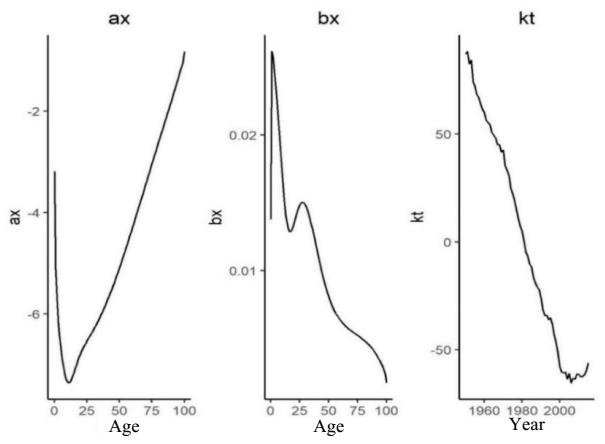
Source: created by the authors with information from CONAPO (2018).
Figure 1 Lee-Carter Model Parameters.
As part of the methodology, the mortality rate κ was analyzed as a time series and adjusted for stochastic modeling purposes using the methodology of Box and Jenkins (1976), finding that an ARIMA (2, 1, 0) process is a good fitting candidate (see Annex 1). After forecasting the 2016-2050 period, the estimated mortality rate for these years is calculated using the values found for parameters a and b. Next, a time series was constructed using the predicted female mortality rates with life expectancies by age for 1950-2050. In the same way, life expectancy was obtained for all age groups between 0 and 100 years during the period. This research assumes that the pensioned population retains the same structure as the group's total population, i.e., each year, people with age x ϵ [65,100] will have a different life expectancy.3 Therefore, within this set, the percentage represented by each subset by age is modified each period. For example, in 2020, people aged 70 will represent 5.75% of the total set; in 2021, 5.76%, and so a different value for each year. In this way, the average life expectancy of the 65 - 100 years group is calculated, weighted by their respective percentage of representation over the total group, annually, for the period 1950-2050.
This determines the weighted life expectancy index, the underlying value for the longevity swaps evaluated in this article. The weighted life expectancy can be interpreted as the annual average of the years remaining to pay a pension to a representative agent of the group of retirees. Monetizing this variable can be understood as the required reserve per pensioner for the year in question for the cost of paying an annuity with a unit value for a total of years equal to the longevity index.
One way to demonstrate that a longevity index is suitable for use as an underlying value in contracts designed for investors in non-retirement sectors is proposed by Friedberg and Webb (2007). Their study shows that longevity risk does not correlate with the S&P500 index.
Similarly, this research indicates that the longevity index developed does not directly relate to various financial market indicators. This confirms that it is a good alternative as an underlying value in derivative instruments for investors seeking to diversify. To illustrate this issue, Table 1 shows the correlation and mutual information coefficients between the annual changes in the longevity index and some representative stock indices of the Mexican and global markets between 1987 and 2015. As can be seen, the trajectories of the main stock indices do not have a significant relationship with changes in the longevity index. This highlights the opportunity for diversification and the use of the index so that different national and international companies find it attractive to join this type of contract, transferring the longevity risk to more liquid markets and demonstrating the feasibility of financial instruments based on longevity.
Table 1 Correlation and mutual information with longevity index (annual rates of change)
Source: created by the authors with information from CONAPO (2018) and Yahoo Finance (2019)
Simulation and valuation of survivorship derivatives and their application
This section presents the main results of this research. First, it simulated a longevity swap for Mexico's PAYG system, left over from the 1997 reform, similar to the one proposed by Rodriguez (2017). Second, it valued several longevity derivative alternatives proposed by Cairns et al. (2010).
Rodriguez's (2017) longevity swap simulation
This subsection presents the simulation of the longevity swap mentioned above with two differences from that proposed by the author. The Lee-Carter mortality estimate developed in the previous section is used instead of the longevity shocks simulated in the author's proportional index, and the monetization variable is also normalized.
For this new swap simulation, the party paying the fixed value delivers an index calculated with the expected mortality table (for this example, the EMSSA-97 table is used). In contrast, the counterparty must pay the real value of the index annually, whose ex-ante value is the longevity index developed in the previous section. Both the fixed weighted life expectancy index and the floating index must be given a monetary meaning for an exchange in financial markets, so that if eX(t) is defined as the weighted life expectancy in year t, the expected reserve per pensioner for the social security system in that period will be:
where M is the pension in force in year t, and φ is the annual rate of change in the value of the pension. Therefore, by obtaining the present value of this obligation (assuming a flat curve of the riskfree rate), this study obtained the value of the premium of a swap maturing in T years, which makes its expected value zero at the beginning of the contract
Where eFix(t) and eFloat(t) are the fixed and floating weighted life expectancies for year t, respectively.
Several assumptions must be made to value this contract. Suppose the Mexican government uses a swap to reduce its exposure to changes in longevity. In that case, it can enter into a contract with a consortium with different exposure to this risk, such as groups of insurers, reinsurers, or unrelated investors. By entering into the contract, the government will pay a fixed amount to its counterparty each year, with no risk of abrupt changes in mortality, and will receive the observed mortality.
Supposing the social security system has an expected annual cost (ex-ante) per pensioner equal to the fixed index of weighted life expectancy during that year, in 2020 the present value of its expected future obligations between 2020 and 2050 will be approximately $3,349, assuming a normalized pension monetary value of M = $1, a flat discount rate of r = 0.055, and annual increments of φ = 0.04 to the pension value. Taking the EMSSA-97 and CONAPO data to calculate the eFloat and eFix indices yield a premium of π ≈ 0.1233 for the swap. Thus, the government would eliminate uncertainty regarding mortality changes by joining a longevity swap in exchange for a 12.33% increase in the present value of its expected obligations from $3,349 to ($3,349 x 1.1233) ≈ $3,762. In comparison, the structuring proposed by Rodriguez (2017) generates a premium of 1.1198%, which shows the sensitivity of the exante cost estimate of a longevity swap.6
To test the degree of risk coverage of the model, 100,000 simulations of the life expectancy index were performed in R Core Team (2018), whose process replicates that of a random walk with drift equal to 0.0536. For this example, two extreme outcomes are chosen: those that presented the highest and lowest longevity increases, taking six scenarios for the Mexican pension system, with swap and without swap, and for both the two extreme scenarios and the central one.
As can be seen in Table 2, the Mexican government can spare itself the uncertainty about the course of mortality in exchange for a premium of $413 (ex-ante) that provides ex-post coverage of 72.1% of the cost in a scenario of an extreme increase in longevity and 64.6% of the cost of an extremely low longevity scenario.
Table 2 Present value of Mexican government obligations (2020 - 2050)
| Scenario | Without swap | With swap |
|---|---|---|
| Increased longevity (ex-post) | $5,221 | |
| Expected longevity (ex-ante) | $3,349 | $3,742 |
| Lower longevity (ex-post) | $2,432 |
Source: created by the authors with information from CONAPO (2018)
Figure 2 shows the trajectory of the swap, presenting the present value of each of its flows during the 31 years of the simulation. In the first years, the fixed part of the swap (social security system) has a loss. However, as of 2031, this situation is reversed, which is reflected in the fact that the sum of the gains or losses (lower line) of this participant in the contract is zero at the beginning of the swap.
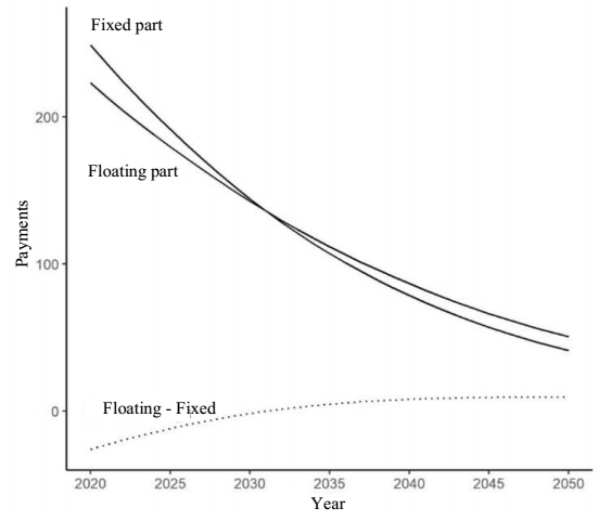
Source: created by the authors with information from CONAPO (2018).
Figure 2 Simulated longevity swap payments for 2020-2050.
Simulation of longevity derivatives from Cairns et al. (2010)
This section evaluates various longevity coverage alternatives proposed in the referenced article, using the data for Mexico and the longevity estimates made in the previous section.
The first alternative to the long-term longevity swap is using a forward swap. In this case, it is assumed as an example that the Mexican government is willing to accept the longevity risk until the year 2030, and from then onwards, it is incorporated into a 2030-2050 swap. In this context, the premium to be covered for the years mentioned above was valued, following the methodology of Cairns et al. (2010).
An ex-ante premium of πfs ≈ 0.211 was obtained so that the present value of the expected future obligations of the social security system would increase from $3,349 to $3,681, which shows that the cost of this coverage is $332 per pensioner.
A second alternative, more attractive to the Mexican government for this type of hedging, is the use of swaptions, which grant the holder the right to enter a swap on the terms specified in the option contract in exchange for the payment of a premium. For example, analogously to the forward-swap, the government can pay to enter a payer swaption in 2030, which would give it the option to enter into the swap as a fixed payer if the swap strike premium specified in the contract is lower than the one in effect at the maturity of the swaption. However, to evaluate longevity options, finding the distribution of the premium π of the survival swap is necessary. Consequently, to realize this goal, 1,000 parametric bootstrap exercises were carried out, where the processes of 1,000 mortality rates κ were simulated as ARIMA (2, 1, 0), thus valuing 1,000 survival swaps and obtaining the distribution of the premium (π) that follows an approximately normal distribution, after which the decision was made to employ the methodology of Dawson et al. (2009).7 Thus, when acquiring a 10-year payer swaption, the government will bear the longevity risk from 2020 to 2029, just as in the forward-swap, but when the option maturity date arrives, if the swap premium from 2030 to 2050 is less than the strike (πfs ≈ 0.211 in this case), the option to participate in the swap would not be exercised and this would be realized in the market, in the usual way. If, conversely, πfs < π, the option is exercised, and the government participates as the fixed payer of a swap with a premium of 0.211. The same values for the necessary variables were used to value the premium for this option, in addition to employing the volatility of the swap premium found equal to σ = 0.2378 for 5 years so that the option would cost 0.1731. Its product is made with the notional value of the payments included to monetize this value in proportional terms, that is, the present value of the part to be received of the swap from 2030 to 2050, where the payment of the floating weighted life expectancy index was established, multiplied by the value of the pension; this is for the representative agent of the group. In this case, the value of the swaption premium is equal to (0.1731 x $1 906.011) ≈ $330, i.e., this contract is a less onerous alternative than the contracts described above.
Paying for this contract has the advantage that when higher mortality scenarios are observed, the social security system can take advantage of this situation without being obliged to deliver a larger amount than is realized. The use of the forward-swap protects in case of an unexpected increase in longevity; however, if there is a decrease in the life expectancy process, the swaption would make it possible to consider the change and would take advantage of this gain in a more efficient way by only paying the premium of $330.
A third alternative is the use of longevity caps. This type of option replicates the hedge provided by survival forwards (which provide the same protection as a long-term swap) but with the right not to exchange flows in the event of a decrease in longevity. It enables the level of weighted life expectancy for each period to be capped at a level pre-specified in the contract by setting the premium that the fixed payer must add at each swap date. For example, if the 31-year swap premium of π ≈ 0.1233 is used as the cap for each period, along with the values assumed above for the rest of the variables, this study values each cap for the 2020-2050 period by employing the premium for each longevity forward as the forward price or premium expectancy instead of the forward-swap premium, which was used in the swaption case.
The effect of having an option of this type is shown in Figures 3 and 4, where it can be observed that in the first years, the expected annual premium is lower than π; therefore, the option is not exercised until it is exceeded, which occurs each year with greater force since mortality is expected to continue to decrease. The second of these figures (Figure 4) illustrates how the cost in monetary terms when using forwards can be decreased through caps-type options. The disadvantage of this type of option is that they are more expensive than other less versatile options, such as longevity payer swaptions; however, in the event of mortality gains, caps would make it possible to take advantage of this situation by a considerable margin since they have this speculative element.
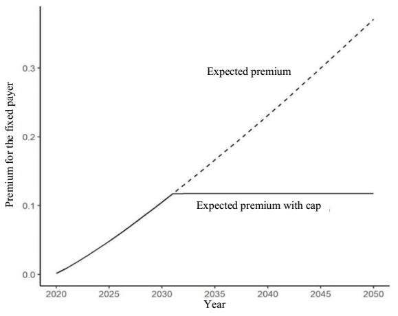
Source: created by the authors with information from CONAPO (2018).
Figure 3 Premium of a survival cap option 2020 -2050.
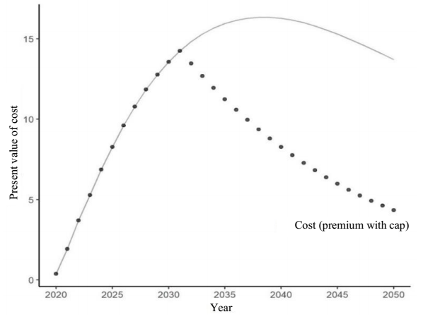
Source: created by the authors with information from CONAPO (2018).
Figure 4 Present value of a survival cap option 2020-2050.
Conclusions
Longevity risk, which encompasses any potential risk associated with the unanticipated increase in the population's life expectancy, can result in greater financial commitments than expected by governments, pension funds, insurers, and individuals. Therefore, its proper management is of considerable importance in advanced and developing economies. The management of longevity risk through financial instruments is a reality in developed countries, with billions of dollars in transactions per year; however, this instrument has not been successfully adopted in undeveloped financial markets.
The results of this research demonstrate the feasibility of using short- and long-term derivative products for longevity risk management with data from Mexico, which contributes to the fulfillment of the general objective of the research, which includes Latin American countries. Although these results cannot be generalized to all Latin America in their present state, the proposed models can be adjusted easily to the data and institutional realities of other countries in the region, such as Brazil, Colombia, and Chile, which can be done in future research projects as part of the consolidation of a line of research.
Concerning the working hypothesis, this is also fulfilled, particularly regarding the feasibility of implementing theoretical and applied developments for longevity derivatives. This is shown in the two strands of the results of this research.
First, a longevity index for Mexico was constructed based on an estimation of the Lee-Carter model. It was demonstrated that this index does not correlate with the main stock indices, which converts it into a potential underlying value for derivative instruments unrelated to financial markets. This implies that national and global investors who wish to hedge diverse risks for financial positions can turn to a longevity market, mainly short term.
Second, the longevity derivatives estimated from this index are effective as hedges of longevity risk. This was shown by structuring and simulating various longevity derivatives. This study started by simulating a long-term longevity swap for Mexico like the one proposed by Rodriguez (2017) but based on the new longevity index, proving that this type of derivative is feasible with the new index proposed here and that they protect the simulated longevity risk adequately. Then, based on the methodology of Cairns et al. (2010), a series of derivatives based on the longevity index proposed were valued, showing that these instruments can be used to realize hedging strategies that transfer the longevity risk of a pension system to different interested participants. Each simulated hedging strategy has its advantages and disadvantages. At the same time, a swap can eliminate longevity risk, and it does not enable speculation on downward movements in life expectancy, which is enabled using high-cost options, which also offer greater flexibility in terms of hedging and investment strategies for different participants.
From these structuring and simulation processes, this study concludes that an ecosystem of long- and short-term longevity derivatives is feasible in a financial market, such as the one existing in Mexico, and that these derivatives can be effective as a longevity risk management strategy for governments, institutions, and individuals. For example, a longevity swap is a long-term contract, usually not very liquid in financial markets. This can make its adoption difficult in the financial markets of medium-developed countries, such as Mexico. However, with a short-term market, the signatories of the long-term longevity swap could discharge their obligations through the short-term instruments proposed and simulated in this article. Thus, it becomes the counterparty to short-term investors seeking non-correlated financial assets.
It is important to consider that the construction of the longevity index proposed here is carried out with an application to the Mexican pension system and that, as proposed by Rodriguez (2017), the use of CONAPO (2018) forecasts regarding the structure of the retirement age group is an important source of base risk that must be observed to be minimized. Likewise, the exemplification of the application of longevity derivatives in this paper uses assumptions that, in practice, could change. However, the reader can undoubtedly adapt with relative ease the models and valuations to fit the reality of the analyzed pension system to give it the greatest realism and the best possible application.
Furthermore, some random variables are involved in structuring longevity derivatives, such as interest rates, changes in pension levels, mortality, fertility, and migration, for which various modeling and estimation methods exist. Therefore, there are always good areas of opportunity in the methodology used regarding its precision and adjustment to reality. One can visualize a space for derivative markets based on different demographic variables, such as fertility and migration.
It is also prudent to point out that there are many more strategies, both simple and complex, whether with risk management and hedging potential or speculation through options and other survivorship derivatives. As presented, these instruments have advantages and a certain appeal for those seeking diversification alternatives in investment portfolios, so it is important to analyze the longevity market from this perspective. The longevity market has great potential and is expected to grow in size and importance as technological, social, and demographic changes continue.
REFERENCES
Alonso, J., Hoyo, C., y Tuesta, J. (2015). A model for the pension system in Mexico: diagnosis and recommendations. Journal of Pension Economics and Finance, 14 (1), 76-112. http://doi.org/10.1017/S147474721400016X. [ Links ]
Balter, A., Kallestrup-Lamb, M. y Rangvid, J. (2021). Macro longevity risk and the choice between annuity products: Evidence from Denmark. Insurance: Mathematics and Economics, 99, 355-362. https://doi.org/10.1016/j.insmatheco.2021.04.009. [ Links ]
Berstein, S. y Morales, M. (2021). The role of a longevity insurance for defined contribution pension systems. Insurance: Mathematics and Economics, 99, 233-240. http://doi.org/10.1016/j.insmatheco.2021.03.020. [ Links ]
Blake, D. (2018). Longevity: a new asset class. Journal of Asset Management, 19 (5), 278-300. http://doi.org/10.1057/s41260-018-0084-9. [ Links ]
Blake, D., y Burrows, W. (2001). Survivor Bonds: Helping to Hedge Mortality Risk. The Journal of Risk and Insurance, 68 (2), 339-348. https://doi.org/10.2307/2678106 [ Links ]
Blake, D., Cairns, A., Coughlan, G., Dowd, K., y MacMinn, R. (2013). The New Life Market. The Journal of Risk and Insurance, 80 (3), 501-557. http://doi.org/10.1111/j.1539-6975.2012.01514.x. [ Links ]
Box, G. E., y Jenkins, G. M. (1976). Time series analysis: Forecasting and Control. San Francisco, EUA: Holden Day. [ Links ]
Broeders, D., Mehlkopf, R., y van Ool, A. (2021). The economics of sharing macro-longevity risk. Insurance: Mathematics and Economics, 99, 440-458. https://doi.org/10.1016/j.insmatheco.2021.03.024. [ Links ]
Cairns, A., Blake, D., Dowd, K., y Dawson, P. (2010). Survivor derivatives: A consistent pricing framework. The Journal of risk and Insurance, 77 (3), 579-596. http://doi.org/10.1111/j.1539-6975.2010.01356.x. [ Links ]
Consejo Nacional de Población-CONAPO. (2018). Bases de datos de Proyecciones de la Población de México y de las Entidades Federativas, 2016-2050. Disponible en: https://www.gob.mx/conapo consultado: 4/08/2018. [ Links ]
Cox, S., y Lin, Y. (2004). Natural Hedging of Life and Annuity Mortality Risks. MIMEO. Departament of Risk Management & Insurance, Georgia State University, 1-25. [ Links ]
Cruz-Aranda, F., Castillo Ramírez, C., y Pérez Flores, C. (2018). Financiamiento del sistema de pensiones mexicano por medio de bonos de longevidad. Revista Mexicana de Economía y Finanzas, 13 (3), 387-417. http://doi.org/10.21919/remef.v13i3.303 [ Links ]
D’Amato, V., Di Lorenzo, E., Haberman, S., Sagoo, P y Sibillo, M. (2018). De-risking strategy: Longevity spread buy-in. Insurance: Mathematics and Economics, 79, 124-136. https://doi.org/10.1016/j.insmatheco.2018.01.004. [ Links ]
Dawson, P., Dowd, K., Cairns, A., y Blake, D. (2009). Options on normal underlyings with an application to the pricing of survivor swaptions. The Journal of Futures Markets, 29 (8), 757-774. http://doi.org/10.1002/fut.20378. [ Links ]
Denuit, M. (2009). An index for longevity risk transfer. Journal of Computational and Applied Mathematics, 230 (2), 411-417. http://doi.org/10.1016/j.cam.2008.12.012. [ Links ]
Dowd, K., Blake, D., Cairns, J., y Dawson, P. (2006). Survivor Swaps. The Journal of Risk and Insurance, 73 (1), 1-17. http://doi.org/10.1111/j.1539-6975.2006.00163.x. [ Links ]
Friedberg, L., y Webb, A. (2007). Life is cheap: Using mortality bonds to hedge aggregate mortality risk. The B.E. Journal of Economic Analysis and Policy, 7 (1), 1682-1785. http://doi.org/10.2202/1935-1682.1785. [ Links ]
García-Guerrero, V., y Ordorica-Mellado, M. (2012). Proyección estocástica de la mortalidad mexicana por medio del método de Lee-Carter. Estudios Demográficos y Urbanos, 27 (2), 409-448. https://doi.org/10.24201/edu.v27i2.1418. [ Links ]
Guerrero, V. (1991). Análisis Estadístico de Series de Tiempo Económicas. Ciudad de México, México: Universidad Autónoma Metropolitana. [ Links ]
Gujarati, D. (2004). Econometría. Ciudad de México, México: McGraw-Hill Interamericana. [ Links ]
Hyndman, R., Athanasopoulos, G., Bergmeir, C., Caceres, G., Chhay, L., O'Hara-Wild, M., y Yasmeen, F. (2019a). Forecast: Forecasting functions for time series and linear models (versión 8.16). Paquete R. Disponible en: https://pkg.robjhyndman.com/forecast/ , consultado: 3/10/2019. [ Links ]
Hyndman, R., Booth, H., Tickle, L., y Maindonald, J. (2019b). Demography: Forecasting Mortality, Fertility, Migration and Population Data (versión 1.22). Paquete R. Disponible en: https://CRAN.R-project.org/package=demography , consultado: 3/10/2019. [ Links ]
J.P. Morgan Chase Bank. (2007). LifeMetrics, a toolkit for measuring and managing longevity and mortality risk. Pension Advisory Group. Disponible en: https://www.researchgate.net/publication/340738356_LifeMetrics_A_toolkit_for_measuring_and_managing_longevity_and_mortality_risks , consultado: 3/01/2020. [ Links ]
Jamal, A., y Quayes, S. (2004). Demographic structure and stock prices. Economic Letters, 84 (2), 211-215. https://doi.org/10.1016/j.econlet.2004.02.004 [ Links ]
Lee, R., y Carter, L. (1992). Modeling and Forecasting U.S. Mortality. Journal of the American Statistical Association, 87 (419), 659-671. https://doi.org/10.1080/01621459.1992.10475265. [ Links ]
Lilien, D., Sueyoshi, G., Wilkins, C., Wong, J.,Fuquay, P., Thomas, G., …Noh, J. (2015). E-views (versión 8.1). IHS Global Inc. [ Links ]
Pfaff, B. (2008). Analysis of Integrated and Cointegrated Time Series with R. Nueva York, EUA: Springer-Verlag. https://doi.org/10.1007/978-0-387-75967-8. [ Links ]
R Core Team. (2018). R: A language and environment for statistical computing. Viena, Austria. Disponible en: https://www.R-project.org , consultado: 19/09/2018. [ Links ]
Rodríguez-Reyes, L. R. (2017). El manejo del riesgo de longevidad en los sistemas públicos de pensiones. Una propuesta de uso de swaps de longevidad para México. El Trimestre Económico, 84 (335), 681-706. https://doi.org/10.20430/ete.v84i335.206 [ Links ]
Stoffer, D. (2019). Astsa: Applied Statistical Time Series Analysis (versión 1.9). Paquete R. Disponible en: https://CRAN.R-project.org/package=astsa . Consultado: 3/10/2019. [ Links ]
Tapen, S. (2012). Estimating future pension liability of the Mexican Government. Inter-American Development Bank. [ Links ]
Yahoo Finance. (2019). Cotizaciones históricas del S&P 500, STOXX 50 e IPC. Disponible en: https://finance.yahoo.com/, consultado: 16/08/2019. [ Links ]
1In order to further boost the longevity market, in 2007 J.P. Morgan structured the LifeMetrics index, based on male mortality in England and Wales, for different age ranges (J.P. Morgan Chase Bank, 2007).
4Hypothesis tests were performed to verify that the calculated Pearson correlations cannot statistically differ from zero (Ho:). In all cases Ho: cannot be rejected at 95%, indicating that the stock indices shown in Table 1 are not significantly correlated with the proposed longevity index. The critical value for n=29 is ±0.367.
5It was calculated by discretizing the rates of change and normalizing with the root of the product of the entropies.
6 Rodriguez's (2017) swap assumes a discount rate of 3.5%, a rate of increase in the number of pensioners of 6%, and a pension growth rate of 4%. His longevity index is also significantly different from the one proposed in this article.
7Normality is determined with the Shapiro-Wilk, Anderson-Darling, and Jarque-Bera tests, with p-values of 0.8791, 0.8219, and 0.7035 for their statistics, respectively.
8The ACF and PACF of 𝐷(𝜅𝑡, 1) provide an additional argument for considering the first difference a stationary series. According to Guerrero (1991), the fact that both functions tend to zero quickly is a sign that there are no unit roots.
Annex
This section shows the analysis of the mortality rate κt as a time series and its adjustment for stochastic modeling purposes using the method of Box and Jenkins (1976), embodied in the methodological proposal of Guerrero (1991). The estimations in this section were performed in the E-views program, version 8.1, by Lilien et al. (2015), yielding an ARIMA (2, 1, 0) model as the best fitting model.
Unit root and differentiation tests
As a first approach to the model, Figure A1, which presents the time series of the level mortality index, κt, is analyzed. This figure shows the need to transform the variable since it does not meet the conditions to be considered stationary in its original state, such as a constant mean and variance over time.
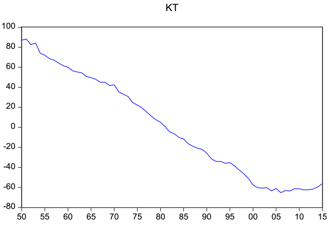
Source: created by the authors with information from CONAPO (2018).
Figure A1 Mortality rate κt, annual graph.
Figure A2 presents the transformed series through the first difference over the original series, D(κt,1). In this case, this is a candidate to be a stationary variable by presenting a non-explosive behavior in mean and variance. The criteria presented in Table A1 confirm that κt is not stationary, and that D(κt,1) is a better candidate for modeling the ARIMA process.
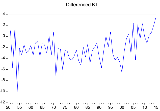
Source: created by the authors with information from CONAPO.
Figure A2 D(κt,1) series; first difference in the mortality rate.
Table A1 Selection criteria for stationary variable
| Variable | Probability Value | Standard Deviation | |
|---|---|---|---|
| ADF | PP | ||
| kt | 1.0000 | 1.0000 | 50.615 |
|
|
0.0830 | 0.0000 | 2.536 |
| D(κt,2) | 0.0000 | 0.0000 | 3.492 |
Source: created by the authors with information from CONAPO (2018)
Table A1 presents the results of two unit root tests, the Augmented Dickey-Fuller test (ADF) and the Phillips-Perron test (PP), and the standard deviation of the original variable and its first and second differences.
Concerning the original variable κt in both unit root tests, the ADF test and the PP test, the null hypothesis is accepted, i.e., it is confirmed that the original series has a unit root, which rules it out as a basis for ARIMA modeling.
In the case of the first and second differences, D(κt,1) and D(κt,2), these present conditions that make them candidates for use in ARIMA modeling. In both cases, the PP test rejects the unit root null hypothesis. However, when using the ADF test, the null hypothesis is rejected in the first difference with a probability value of 0.0830, marginally above the conventional critical level of 0.05. In contrast, the ADF test for the second difference yields a probability value within the conventional rejection zone.
These results demonstrate the need to carefully decide the level of differentiation to be used in the model. Both options present arguments for and against, but the main criterion for choosing the first difference is to avoid over-differentiation. This causes problems in the model identification, increases the series’ variance, and causes a loss of observations (Guerrero, 1991: pp. 24-25). A clue to determine that the second difference implies over-differentiation is the increase in the standard deviation of the series concerning the first difference. This criterion, together with the results of the PP test, leads to choosing the first difference, D(κt,1), as the base variable for the ARIMA modeling.
Model choice: Autocorrelation functions and ARIMA model estimation
To propose ARIMA models as candidates to represent the behavior of 𝐷(𝜅𝑡,1), the autocorrelation functions (ACF) and partial autocorrelation functions (PACF) of the series, presented in Figure A3, are analyzed. From the behavior shown in both functions, this study concludes the possible existence of autoregressive (AR) or moving average (MA) components, both of order 2. Both functions rule out the existence of AR and MA components of different orders. Therefore, the ARIMA (2,1,2) model is initially proposed.8
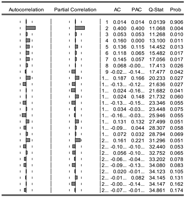
Source: created by the authors with information from CONAPO (2018).
Figure A3 D(κt,1); autocorrelation and partial autocorrelation functions.
Next, the ARIMA (2,1,2) model was estimated using the ordinary least squares (OLS) technique, the results of which are presented in Table A2. According to the statistical significance analysis of the coefficients, the one corresponding to the moving average term, MA(2), cannot be statistically distinguished from zero, so an alternative ARIMA (2,1,0) model was estimated for comparative purposes, the results of which are also included in Table A2.
Table A2 OLS estimation of the ARIMA model of D(κt,1)
| ARIMA Modelo | Coefficients (P-value) | Schwartz Criteria | ||
|---|---|---|---|---|
| C | AR(2) | MA(2) | ||
| (2,1,2) | -1.875646 (0.0039) |
0.709221 (0.0000) |
-0.404809 (0.0612) |
4.581600 |
| (2,1,0) | -2.063437 (0.0003) |
0.458115 (0.0003) |
4.574966 | |
Source: created by the authors with information from CONAPO (2018); sample 1953-2015 (annual data)
Both ARIMA models could be used to construct forecasts for the variable κt; however, the ARIMA (2,1,0) model is chosen using the possible overspecification of the ARIMA (2,1,2) model as a criterion. Including an unnecessary variable in the model causes the coefficients estimated through OLS to be generally inefficient, i.e., their variances are larger than those of the true model (Gujarati, 2004). This would necessarily imply higher variance ranges for forecasts using the ARIMA (2,1,2) model, which goes against the fundamental purpose of this modeling. In the case of the ARIMA (2,1,0) model, one can be confident that it is not overspecified by having the two model coefficients statistically different from zero. Additionally, in terms of the Schwartz criterion, by eliminating the MA(2) term from the original model, there is a gain in the quality of the information. Therefore, it is concluded that the ARIMA (2,1,0) model is the best model for the D(κt,1) series.
Residual tests and forecasts
Once the ARIMA (2,1,0) model was chosen, three tests were performed on the model's residuals: the Jarque-Bera test for normality, and two serial correlation tests, the Ljung-Box test, and the Breusch-Godfrey LM test. In the case of the Jarque-Bera test, the null hypothesis (𝑝 = 0.45325 > 0.05) is accepted, so the residuals are normal. In the case of the serial correlation of the residuals, in both tests the null hypothesis is accepted, confirming that there is no serial correlation in the residuals of the ARIMA (2,1,0) model. In the Ljung-Box test 𝑝 ∈ [0.142, 0.85] > 0.05 for all 28 lags used, while in the Breusch-Godfrey LM test 𝑝 = 0.0779 > 0.05.
The estimated ARIMA (2,1,0) model is algebraically transformed into Equation 6, which is used to make forecasts of the 𝑘𝑡 variable starting from the last annual data of the series and up to 2050.
The forecast estimation is presented graphically in Figure A4, where it may be noted that the historical trend of 𝑘𝑡 is expected to continue as the central value; however, a lateral behavior is also possible since this scenario is within the confidence interval formed by the positive and negative values of twice the standard error.
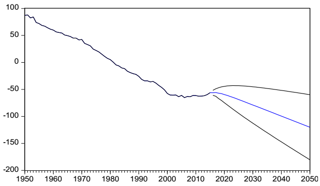
Source: created by the authors with information from CONAPO (2018).
Figure A4 Forecasts of the kt series.
Finally, these forecasts are fed into the Lee-Carter model to construct the longevity index used in this study's estimations and valuations of the longevity derivatives modeled for Mexico.
Received: April 01, 2021; Accepted: May 13, 2022; corrected: June 17, 2022
 Este es un artículo publicado en acceso abierto bajo una licencia Creative Commons
