


 text new page (beta)
 English (pdf)
 Article in xml format
 Article references
 Send this article by e-mail
 Cited by SciELO
  Similars in
SciELO
Similars in
SciELO 
 Permalink
Introduction
Predicting the volatility of the exchange rate in the short term is undoubtedly a challenge for heavily traded emerging markets, which are subject to natural speculation against less volatile currencies in the short term. The Mexican peso (MXN) is the tenth most traded currency in the world. The daily turnover of the peso oscillates around USD 112 000 million and 97% of these transactions are made against the US dollar. The latter currency had a total trading volume of all currencies of 87.6% in 2016.1
In the Mexican current account in the first quarter of 2016 imports reached USD 89 133 million and exports were USD 85 148 million.2 The amount of Mexican pesos that moves over two days in the foreign exchange market is much greater than the exports and imports combined in a single quarter; this is a key factor in the exchange rate being subject to speculation within the market currency.
Moreover, purchasing power parity (PPP) considers the exchange rate as a price; (Taylor & Taylor, 2004) demonstrate that PPP shows deviations from the expected value in the short term. The price or exchange ratio can be considered a demand variable, which is influenced by the external market of goods, the financial market (derivatives), and its own market: the exchange rate (the variable itself generates its own dynamics) and the speculation of this same market. It is necessary to take into consideration that in the short term not all variables play an important role in the supply-demand relationship for foreign exchange.
The financial system has become very complex and this has led to different social science fields, such as psychology and neuroscience, wondering how financial decisions are generated. They consider that financial decisions happen at different levels of aggregation as opposed to economic theories. (Frydman & Camerer, 2016) mentions the example of the efficient market hypothesis, which only takes into account data from market levels, leaving aside information from individuals.3
(Frydman & Camerer, 2016) find four levels of aggregation: (i) household, (ii) individual trading patterns, (iii) decisions that determine the price of assets in the market, and (iv) corporate investment funds. Data from search engines may belong to more than one level of economic aggregation, although it is difficult to distinguish to what level they belong; nonetheless, part of the results obtained herein provide us with an idea, as mentioned below. Google Trends should belong to (i) or (ii) above, because (iii) and (iv) may well use other specialized sources of information, such as Bloomberg.
Empirical studies have proposed a number of simple models to explain economic variables using Google Trends. For example,(Choi & Varian, 2012) use autoregressive (AR) models to forecast auto parts sales, tourism, and unemployment. They find that Google Trends are often correlated with economic indicators and are useful for improving short-term prediction as they attain the most successful outcomes at breakpoints or inflection points. In addition, (Carrière-Swallow & Labbé, 2013) find that the AR(1) model has a very good fit and produces more successful results outside the sample than considering other higher order specifications. They also analyze consumer behavior, i.e., interest in buying a car, by building an indicator that involves Google Trends.
Other models are based on the similarity function, which most closely resembles the natural form of human reasoning. According to (Lieberman, 2010), this function can be used to predict the variable in question, taking into account similar information and the same historical variable, as proposed by (Gilboa, Lieberman, & Schmeidler, 2011). One example is an economic analyst who needs to forecast next year’s inflation. Some current applications of the similarity function have been to explain the volatility of the stock exchange (Golosnoy, Hamid, & Okhrin, 2014), and of even greater relevance to this work, it has been used to explain volatility using Google’s search engine trends (Hamid & Heiden, 2015). The latter authors find that in short periods of high market volatility, prediction improves when investors’ attention to the market is taken into account if Google Trends are used.
The Google search engine is the one most used worldwide, embracing 67.78% of the desktop market, and on mobile devices and tablets 94.4% of the market see (Market share, 2017).
The objective of this paper is to develop different methodologies to examine the MXN- USD exchange rate variable. On the one hand, there are models based on AR, using time series that directly incorporate the trend; on the other hand, there are models based on the similarity, which performs a transformation, as shown in section Empirical volatility models.
Theory and literature review
The use of big data indicators in economics is growing. (Guzmán, 2011) uses Google Trends to forecast inflation. (McLaren & Shanbhogue, 2011) propose that the data generated by a web search can be used by central banks in the management of economic nowcasting. (Carrière-Swallow & Labbé, 2013) use this means for auto sales nowcasting in emerging markets (Smith, 2012) investigates if the activity of the search engines is related to the volatility of the foreign exchange market. Specifically, he takes into consideration the search terms: economic crisis, financial crisis, inflation, and recession. With these terms in Google Trends, he constructs two estimators, one over the short term and one over the long term, for which he considers a four-week moving average. He employs these short-term and long-term estimators in three different ordinary least squares models, incorporating volatility for seven currencies. However, the R2 statistics are poor considering the use of three variables to explain volatility in all cases and one intercept. It is thought that this may be due to the fact that the search terms chosen are somewhat technical and it is not known whether there is an empirical correlation of these terms with the volatility variable to be explained. Moreover, there is a question concerning whether these particular Google Trends capture the real behavior of investors. Nonetheless, the author concludes that these keywords can predict volatility in the foreign exchange market, albeit they only capture part of the volatility of the entire market of financial decisions that spin around the currency market.
(Hamid & Heiden, 2015) forecast volatility by incorporating Google Trends to forecast the variance of the Dow Jones index based on five-minute returns, focusing on weekly forecasts.
On the other hand, GARCH family models are widely used to analyze volatility. (Kumari & Mahakud, 2015) built a sentiment index to analyze the return on assets of the Indian market. They incorporated the index in the mean and variance of the GARCH model. They find that their sentiment index helps to anticipate negative and positive return volatility.
(Afkhami, Cormack, & Ghoddusi, 2017) looked for terms in the Google engine that best represented market investors in order to forecast energy price volatility. They used ninety search terms related to the energy market and they contrasted them with the usual GARCH.
(Morimoto & Kawasaki, 2017) modelled market volatility taking into account on line intraday news using HAR models, big data techniques and text mining techniques.
Other authors suggest that investor attention is a driver of volatility over short periods of time (Vlastakis & Markellos, 2012), and that there is a close relationship in phases of high volatility (Andrei & Hasler, 2015).
In this paper, we use Google Trends data as volatility variables in relation to the exchange rate because people’s interest when looking for relevant information concerning a financial economic variable can be translated as a precursor or an indicator of whether there is volatility in that variable and considering this as one direct variable in the model would imply a lower final impact of this variable. (Alvarez, Atkeson, & Kehoe, 2007) consider that in the short run, the exchange rate is not affected in the first statistical moment; they propose a theoretical model in which they analyze the effects of the second statistical moment on the currency.
Empirical volatility models
According to (Gilboa, Lieberman, & Schmeidler, 2006), there are sometimes issues to be solved that are unique, such as calculating the sale price of a work of art, knowing if a person’s body will react successfully to a certain operation, or an analyst determining the rate of inflation for the following year. Thus, sometimes the information is not sufficiently relevant to explain a particular case and it is sometimes necessary to weigh the information, counting it and assigning it a weight according to its importance for the case under study. This seems a more accurate approach than simply taking all available information directly and expecting it to suffice to answer the issue that the analyst wishes to address; in this context considering “similar” variables adopted in other studies can improve the prediction process. Economic agents prefer to obtain good results based on similar cases that have previously been well adjusted.
Mathematical models that incorporate cognitive processes, observed behaviors, and novel data sources generated by individuals or the economy are considered models of economic behavior. These types of predictive models are formulated using the similarity function see (Gilboa et al., 2011). (Lieberman, 2010) argues that the similarity function can be considered a natural model of human reasoning and its statistical validity has been shown through the axioms of (Gilboa et al., 2006).
We define the process of exhibiting interest yt+1 as follows:
with εt ~ (0, σ 2).
(Golosnoy et al., 2014) interpret x i,t-1 as previous forecasts similar to y t . The variable x i,t-1 must naturally be similar to y t in the past. For this reason, the distance between the two must be small, so as to give:
The forecast is given by:
The similarity function is represented by a Euclidean distance
The concept of “similarity” can be extended to analyze volatilities. This would imply that yi must be a known volatility variable to be forecast, and the similarity function must be constructed with variables that can anticipate future volatility behavior based on past behavior; in line with this, the economic agent will take the information and consider it in accordance with the function of similarity to construct the estimate of the volatility that will arise in the future.
The similarity function is specified as:
where G i,t-1 is the trend behavior variable generated by the individuals.
Temporal models
The random walk can be represented by an AR(1) process. (Charles R. Nelson & Charles R. Plosser, 1982) analyze different macroeconomic series, concluding that the best prognosis for these is very close to the random walk. In different works, it has been established that for the main currencies a random walk can be a good approximation of the nominal exchange rate.
The simpler model proposed by (Choi & Varian, 2012), based on time series, follows the following dynamic:
With e t ~ (0, σ 2). Where y_t is the process to be explained, gt the variable corresponding to Google trends, and b 12 y t-12 the seasonal component, if this exists.
Data
Google trends data
Google Trends data are collected through the company’s search engine; this collates relevant searches for any topic browsed on one’s page and that can be downloaded from the (Google, 2017b) web page. The data are standardized by the keywords that generate the highest number of searches on a specific date. This value represents 100% and the other values for data must be lower than this amount.
The Google Trends website allows one to view and download up to five joint variables, but one must be very careful because when they are downloaded together, they are standardized based on the most searched variable. If the query is downloaded in isolation, it is standardized based on the most searched data. It is possible to select the data by region of the world and choose the temporal frequency. It is also possible to select where one looks for the topic of interest: in the web browser, in the image finder, or in the news. Moreover, it also allows one to visualize geographically the countries represented in the search area, shading the most important regions in navy blue and the less important in light blue in terms of the total number of searches.
We use historical data for the trend of the “precio dolar,” counted weekly beginning in the week 04/01/2004 to 10/01/2004 and ending in the week 03/20/2016 to 03/26/2016 (639 observations). The observations begin on Sunday and end on Saturday. The process of choosing the “precio dolar” variable is as described in Annex A. In terms of the selection of trend variables, the geographical area was not delimited, the intention being to visualize which countries are interested in acquiring USD and what might start speculation in demand for USD, i.e., what would motivate more foreign investors to purchase this reserve currency, or simply to reflect the behavior of an entire area that might acquire USD, directly affecting the MXN-USD exchange rate.
Exchange rate data
The historical data for the exchange rate were downloaded from the Banco de México (BANXICO, 2017) portal; the information is daily from January 1, 2001 to March 29, 2016. The data for Fridays are taken as the closing values of the exchange rate price in each week, so that the data are weekly and are homogeneous with the weekly trend data.
Realized volatility of the exchange rate
Realized volatility refers to volatility that occurred in the past and usually concerns derivatives. For example, if we wish to examine monthly volatility, it can be calculated by taking the standard deviations of the daily returns in the desired month according to the (Nasdaq, 2017) website.
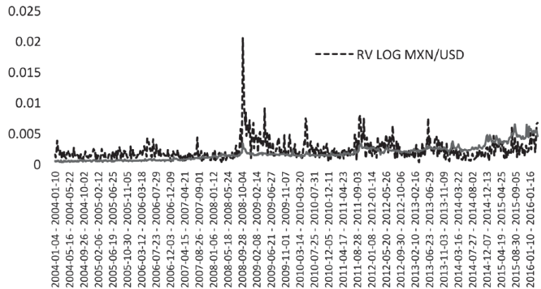
Source: Own estimation with data for the MXN-USD exchange rate and the variable “precio dolar” in Google Trends; both variables are on a similar scale. (2004-2016)
Figure 1 Realized volatility of the log exchange rate, MXN-USD, against Google Trend data. (2004-2016).
For the second time (the first being in the selection of trend variables), we use Granger’s causality test on the realized volatility and the Google Trends variable, finding that in its first and sixth lags in the test, the Google Trends variable Granger causes realized volatility with a significance level of 5%.
It should be noted that the data, even for the past, are updated according to the maximum value recorded in the specified period of time. For example, in a future period when a higher query volume for a search term is registered than in the previous data, this maximum modifies all the series, adjusting them with the new value. In considering a specific range in the past that does not consider the present period, clearly in that time range the maximum search value will be different.4 Thus, when considering a fixed data series, it is incorrect to consider dividing the series within the sample. It would only be valid if the maximum value of the whole series were considered in the same range within the sample, or another series were downloaded for the selected period; this might change the specification of the model that takes the present into consideration. We consider that the best option is to perform contrasts outside and not within the sample.
Methodology and results
According to (Choi & Varian, 2012), trend variables can be incorporated directly into the model. Applying the same idea to explain realized volatility, we have the following:
In this specification, all coefficients are found to be significant and the standard error has a level consistent with the coefficients see Table 1.
Table 1 Parameters of the time series of volatility.
| Coefficient | Standard Error | t value | Pr (>|t|) | |
| Intercept | 0.00130 | 0.00042 | 3.09019 | 0.00224 |
| b 0 | 0.39596 | 0.12528 | 3.16068 | 0.00178 |
| b 1 | 0.42051 | 0.05292 | 7.94531 | 7.51E-14 |
| Adj R-squared: 0.2093, AIC: -10.5437 | ||||
Source: Own elaboration.
On the other hand, the empirical similarity (ES) method is not interested in directly analyzing the variables over time. The methodology tries to weigh similar cases to improve the forecast. This feature is an advantage when the historical information does not exhibit regular and consistent periodicity in the entire sample.
Here, we adopt a variation of the ES methodology, as described by (Hamid & Heiden, 2015):
RV t and RW t =exp(-ω 1 (RV t -G t )) RV t are weakly stationary in booth models. Table 2 reports our results of unit root tests (Dickey & Fuller, 1979, 1981) and (Phillips & Perron, 1988).
Table 2 Unit root tests in levels.
| Variable | Unit root tests(Level) | Test statistic | 1% Critical value | 5% Critical value | 10% Critical value |
| RV t | Dickey-Fuller(DF) | -3.65289 | -3.457061 | -2.87319 | -2.573054 |
| Phillips-Perron(PP) | -10.8164 | -3.457061 | -2.87319 | -2.573054 | |
| RW t | Dickey-Fuller(DF) | -3.89707 | -3.457061 | -2.87319 | -2.573054 |
| Phillips-Perron(PP) | -11.19332 | -3.457061 | -2.87319 | -2.573054 |
Source: Own elaboration.
Table 3 shows the values of the parameters obtained for the ES model; the Akaike information criterion (AIC) is quite similar in both models. Interestingly, the significance level of the second model is preferable based on the values of the t-statistic.
Table 3 Parameters of the empirical volatility model.
| Coefficient | Standard Error | t value | Pr(>|t|) | |
| Intercept | 0.00091 | 8.86E-05 | 10.29908 | 4.16E-23 |
| b 1 | 0.58949 | 0.03244 | 18.17408 | 9.61E-60 |
| Adj R-squared: 0.3421, AIC: -10.4203 | ||||
Source: Own elaboration.
Figure 2 shows the out-of-sample auto one-step-ahead predictions with fixed coefficients. The period visualized is from April 4, 2016 to October 29, 2016; as we can see, both methodologies fail to capture the full magnitude of the volatility, leading us to believe that the financial decisions that are reflected only represent a part of the total behavioral decisions within the foreign exchange market.
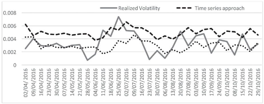
Source: Own elaboration with Banxico and Google Trends data. (2016)
Figure 2 Out-of-sample; realized volatility; time series approach and ES approach. (2016).
The ES approach follows the real volatility more closely, but it does not capture the full breadth of the volatility or its shape.
In Figure 3, the behavior shown by investors before the historical maximum of the MXN- USD exchange rate shows no considerable variation. If we undertake a visualization using a window of more years, it is clear that there is no change in tendency in the series over the period. In Table 4, we can confront this with the real values of the exchange rate. Over time, interest only increases highly from September 19, 2016 to September 20, 2016 (see Figure 3) and from September 21, 2016 to September 26, 2016 the interest rate is down. In this last period, higher values of the MXN-USD exchange rate are achieved.
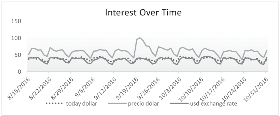
Source: Elaborated using the Google Trends portal for the keywords “today dollar”, “precio dolar”, and “USD exchange rate”. (2016)
Figure 3 The MXN achieves its maximum historical value of USD 19.83 (MXN/USD) on 09/21/16. (2016)
Table 4 Variation in the MXN-USD exchange rate in the month of September.
| Daily Date | USD/MXN |
| 07/09/2016 | 18.3689 |
| 08/09/2016 | 18.5427 |
| 09/09/2016 | 18.8451 |
| 12/09/2016 | 19.0646 |
| 13/09/2016 | 19.152 |
| 14/09/2016 | 19.2275 |
| 15/09/2016 | 19.2514 |
| 19/09/2016 | 19.6097 |
| 20/09/2016 | 19.777 |
| 21/09/2016 | 19.8394 |
| 22/09/2016 | 19.5965 |
| 23/09/2016 | 19.7211 |
| 26/09/2016 | 19.8322 |
Source: Own elaboration with data of BANXICO.
Note: In this period, there is no marked prior interest for different keywords; only on 09/19/2016 and 09/20/2016 does it show a sudden interest, but this disappears quickly.
Conclusions
The way in which the volatility of the MXN-USD rate is modeled in this work is quite novel because it incorporates the behavior of individuals in different regions of the world whose financial decisions are focused on acquiring USD, possibly to avoid a devaluation in capital, or simply to try to generate profits by anticipating the depreciation of an emerging country’s currency. All this directly affects the Mexican peso in the short term. The similarity model represents a clear way of capturing such behavior. Even so, a lot of work remains to be done; in particular, it is necessary to include more relevant variables for short-term impact.
For example, in the results obtained, even in the most volatile periods it is not possible to capture the behavior of all the investors. Examining different variables in Google Trends, they do not reflect drastic upward movements in the month of September 2016 (see Fig. 3), which makes us think that there are different levels of economic aggregation at which different financial decisions are made. Moreover, the Google Trends variable only represents a part of the financial decisions that are made in the currency market.
An extension of this study would be to determine what sources of information allow us to anticipate the behavior of big capital, which surely comes from large corporate investment funds and cannot be captured by the Google Trends volatility proxy chosen here.

