


 text new page (beta)
 English (pdf)
 Article in xml format
 Article references
 Send this article by e-mail
 Cited by SciELO
  Similars in
SciELO
Similars in
SciELO 
 Permalink
Introduction
Most of the studies in finance has extensively used different factor model to understand the risk return relationship. These factor models are generally linear in nature by linear it means the dependent variable are linearly dependent on the independent variable. Financial data generally have fat long tail and OLS regression at the end tails become ineffective. The financial factor models are OLS regressions and OLS is based on the mean value of the covariates and hence it is ineffective in the end distributions. Tail values are of more significance to the analyst and risk managers as they have to make investment decision. Decision based on OLS results mostly lead to wrong decision, to address the same Quantile regression is used in evaluating these extremes of the distribution and compared with the OLS results. In this paper 10 value sorted portfolios returns are analysed using the Fama-French (1993) model using the OLS and Quantile regression methods exclusively to test value effect.
Review of literature
As earlier discussed most of the studies in finance extensively used OLS regression for different factor models and none of the previous financial studies with factor models has critically addressed whether the factor model is effective in capturing the tailed distribution results or not? As in most cases the financial data consists of fat tails and in the tail part the distribution generally do not follow normal curve distributions. Ordinary least square regression follows the central tendency theorem and more effective at the median of the distribution. Towards the extreme distributions it loses its effectiveness and due to which result may not be correct. Embrechts, Kl¨uppelberg & Mikosch (1997) study used the extreme value theory (EVT) and EVT then used for the extreme events analysis of floods, extreme temperatures, winds and finance. Many researchers like Marinelli, D’Addona & Rachev (2007), and Sheikh & Qiao (2009) have extensively used the extreme value theory to their financial research to tackle the extreme events. For modelling two different methods namely the block of maxima method and peaks over threshold method are used. Again there lies disadvantages lies with both the approaches to counterfeit it Zumbach (2006) study suggests some modelling technique to deal with this thick tails. Rachev (2003) in his book clearly explains about the heavy tail distributions in finance and the difficulties associated with it. Then it discussed about some probabilistic and statistical models like non-Gaussian to overcome such problem. Recent study by David, Abhay and Robert (2011) and Dutta & Biswas (2017) study confirms that financial tail data need special attention. It is clear that financial data do have fat tails and over the period of time different researchers has followed different methodology to overcome it but unable to capture as a whole.
Most of the studies in finance only use factor model or regression techniques. So, there are possibilities that the study result has error especially at the end distributions. These are few of the notable studies where the researchers have raised several questions regarding the factor model usage in the financial studies. Fama-French results were tested by the Black (1993) and the study finds that the size effect is due to the data mining effect rather than what is quoted in the study. Kothari, Shanken and Sloan (1995) find that different frequency of data yield different result for the beta effect and it is more prominent for the annual data. Similar result also finds by the Levhari and Levy (1977) study that beta coefficients do differs for the annual and monthly data. Kenz and Ready (1997) study find after trimming the 1 % tailed data using the least trimmed squared techniques (LTS) the size effect greatly reduced. From all of the above studies and several other studies that are not mentioned provides sufficient evidences about the stocks returns move off from normality and shows fat tail distribution. The size effect is also not constant for whole study period. For the present study uses the more vigorous method of Chan and Lakonishok (1992).
Data and Methodology
Data
The present study uses monthly data of the BSE 500 stocks for the period from Jan 2003 to April, 2015. Stock returns are calculated from the closing share prices of stocks. Market capitalisation (MC) is used as the proxy for size and Price to book ratio (P/B) is used as the proxy for value. BSE-200 index monthly excess return taken as the proxy for market returns and all of the above mentioned data are collected from the Bloomberg database. 91day T-bill returns are used as the proxy for the risk free rate of return (Rf) and it is collected from the database of Reserve Bank of India (RBI).
Portfolio construction
10 weighted portfolios (each 10 %) are constructed by P/B ratio sort using the single sorting techniques (Portfolios are named as Low, 2 to 9 and High). Mimi kicking portfolios are constructed using the Fama-French (1993) methodology using both the single and double sorting techniques as explained below. SMB1 and LMH2 (LMH used instead of HML in FFTF regression, see Sehgal, S., Subramaniam, S., & De La Morandiere, L. P. (2012)) are mimicking portfolio for size and value factors. By single sorting technique two value weighted market capitalisation (MC) portfolio of ratio 90:10 are constructed. Then using the double sorting techniques six portfolios are constructed from the cross of 2 size and 3 value sorted portfolios. Portfolio S/L consists of small size and low P/B ratio companies; similarly Portfolio B/H consists of big size and high P/B ratio companies; rest are named as S/M, S/H, B/L & B/M based on acesending order of MC and P/B. Hence, every June moth of each year (t) portfolio is ranked. Then each portfolios value weighted monthly excess return calculated for the period of July, 2003 (t) to June, 2004 (t+1). In the similar process the next ranking done for the year 2004 and continues till 2015. Then for the whole period of 156 months from July, 2003 to April, 2015, means excess returns on each portfolio are calculated. The formula for calculating SMB and LMH are shown below:
Study uses Fama-French three factor models as discussed below:
Where,
SMB mimics the risk factor in returns considering size
LMH mimics the risk factor in returns considering value
s and l are the portfolio’s responsiveness to (sensitivity coefficients) SMB and LMH factors respectively.
Quantile regression
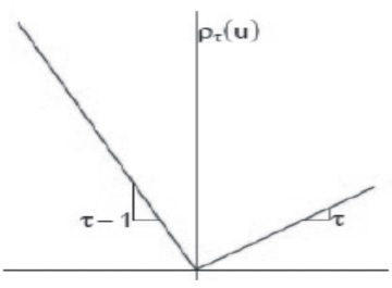
Quantile regression is introduced by Koenker and Bassett (1978). It is based on the conditional Quantile functions that estimate the conditional median or the conditional quartile of the dependable variables for the given independent variables. It is quite similar to the OLS regression as in OLS change in the coefficients of the independent variables denotes the change from one unit change of the predatory variables associated with; in case of Quantile regression it is the change of coefficients with changes in the specified Quantile from one unit change of the predatory variables associated with it. Quantile divides the data into equal percentiles and is more robust in capturing the outliers effectively. Quantile regression uses the median estimator that reduces the sum of absolute errors to estimate the median function. Similarly for other conditional Quantile function of interest (as in our case 0.05 and 0.95) is estimated by reducing the asymmetric weight of absolute errors, where weights are function of the Quantile for interest. In other words it can be said that Quantile are the optimization problem. Sample mean can be defined as the solution to the problem of reducing the sum squares of residuals; similarly the median can be defined as the solution to the problem of reducing the sum of squares of absolute residuals with an aim to reduce the sum of square of residuals or absolute errors. Sum of absolute residuals is said to be minimised when there is equal number of positive and negative residuals lies above and below the median line. Similarly other quintile functions can be obtained by giving different weights to the negative and positive residuals, i.e., by minimising the asymmetric weights of the residuals. In statistics or mathematical notations loss function is defined as follows:
The Ʈth quartile ξ minimises as shown in below equation (Univariate):
The above function has bidirectional derivatives and is not differentiable:
Right derivative
Left derivative
At point ξ minimizes the objective function if R´ (ξ+) ≥ 0 and R´ (ξ-) ≥ 0
The optimised problem defined the unconditional Quantile above in the similar way the conditional Quantile can be defined analogously by OLS as explained below.
[Y1, Y2……….Yn] is a set of random variable from it, we get
Unconditional population mean is estimated from Equation 8. Then the parametric function µ (x, β) replaces the scalar µ in the above equation, we get Equation 9.
Similarly conditional median function can be obtained by replacing the scalar variable ξ by the parametric function ξ (xt, β) and by setting the Ʈth quantile as 1/2. Other condition functions values can be obtained on replacing absolute values by ƍT(*), we get as follows:
Further using linear programming the minimising problem can easily be solved by formulating ξ (x, β) as linear parameters.
In several areas of economics and other sciences this method has been used extensible in past. Some of the notable studies are done to investigate the wage structure (Bunchinsky and Leslie (1997)); educational attainment (Eide and Showalter (1998)); earnings mobility (Eide and Showalter (1999), Buchinsky and Hahn (1998)). Similarly in finance several notable studies are done related to VaR and options (Engle & Manganelli (1999) and Morillo (2000)); CAPM (Barnes & Hughes (2002)); Fama-French three factor model (David, Abhay and Robert (2011)) etc., extensively using the same methodology.
Explanatory variables
The Table 1 below shows the descriptive statistics of all the variables. Weak value effect is observed in the portfolio returns as shown below in Table 1. Investor those who are investing in the portfolios based on P/B is certainly not going get very less value premium. Hence, investor shouldn’t consider P/B as the best indicator to construct the portfolios. For portfolio construction other measures like size, investment, profitability, liquidity etc., or a mix of these variables can be considered.
Table 1 Descriptive statistics
| Portfolios | Mean | Median | Max. | Min. | Std. Dev. | Skewness | Kurtosis |
| Low | 0.025 | 0.023 | 0.438 | -0.299 | 0.092 | 0.297 | 2.682 |
| 2 | 0.024 | 0.031 | 0.474 | -0.308 | 0.093 | 0.665 | 3.846 |
| 3 | 0.026 | 0.024 | 0.473 | -0.279 | 0.097 | 0.385 | 2.522 |
| 4 | 0.024 | 0.025 | 0.427 | -0.309 | 0.096 | 0.261 | 2.524 |
| 5 | 0.028 | 0.029 | 0.444 | -0.290 | 0.095 | 0.337 | 2.459 |
| 6 | 0.027 | 0.024 | 0.425 | -0.303 | 0.091 | 0.177 | 2.644 |
| 7 | 0.022 | 0.023 | 0.420 | -0.276 | 0.087 | 0.176 | 2.797 |
| 8 | 0.026 | 0.028 | 0.467 | -0.297 | 0.096 | 0.310 | 2.879 |
| 9 | 0.023 | 0.025 | 0.457 | -0.301 | 0.096 | 0.274 | 2.581 |
| High | 0.026 | 0.032 | 0.488 | -0.286 | 0.094 | 0.525 | 2.877 |
| Rm | 0.006 | 0.004 | 0.318 | -0.276 | 0.075 | -0.093 | 3.680 |
| SMB | 0.025 | 0.016 | 0.221 | -0.177 | 0.064 | 0.334 | 3.078 |
| LMH | -0.007 | -0.009 | 0.262 | -0.403 | 0.061 | -1.243 | 3.461 |
Empirical results
Below in Table 2 shows Fama-French Three factor coefficients obtained from both OLS and Quantile regression (5th Quantile & 95th Quantile). OLS result shows all SMB coefficient positive whereas the coefficient obtained from Quantile regression at 0.05 Quantile shows negative coefficient for portfolio number 4. That implies that at the lower quartiles relationship between size and return is negative but it becomes positive in the higher quartiles. Hence, one will make wrong decision if the decision is based on OLS regression only. Similar result observed for portfolio number 4 in case of LMH coefficient where OLS result shows negative coefficient for LMH but LMH coefficient obtained from Quantile regression at 0.95 Quantile is positive. Here it implies that at the lower quartiles relationship between value and return is positive but it becomes negative in the higher quartiles. Further the study result find similar such observations and that are shown by * in the Table 2. This clearly evidences the fallacy of OLS regression in the tail part.
Table 2 Fama-French Three factor coefficients obtained from OLS and Quantile regression (5th Quantile & 95th Quantile)
| OLS | Quantile (5th) | Quantile (95th) | ||||||||||
| Portfolio | C | Rm | SMB | LMH | C | Rm | SMB | LMH | C | Rm | SMB | LMH |
| Low | 0.013 | 1.126 | 0.193 | -0.051 | -0.033 | 0.987 | 0.137 | 0.052* | 0.067 | 1.275 | 0.359 | -0.322 |
| T-value | 4.150 | 28.472 | 4.187 | -1.057 | -7.056 | 23.271 | 2.076 | 0.462 | 10.272 | 27.812 | 5.522 | -2.825 |
| 2 | 0.010 | 1.092 | 0.266 | -0.250 | -0.036 | 0.982 | 0.183 | -0.260 | 0.060 | 1.144 | 0.385 | -0.369 |
| T-value | 2.965 | 26.791 | 5.594 | -4.988 | -6.530 | 14.662 | 1.528 | -2.333 | 11.063 | 29.744 | 7.077 | -12.67 |
| 3 | 0.016 | 1.167 | 0.160 | 0.059 | -0.037 | 1.125 | 0.032 | 0.089 | 0.092 | 1.389 | 0.320 | 0.018 |
| T-value | 4.143 | 24.538 | 2.897 | 1.009 | -8.171 | 16.574 | 0.537 | 2.001 | 7.788 | 19.511 | 3.560 | 0.200 |
| 4 | 0.014 | 1.156 | 0.153 | -0.011 | -0.046 | 0.933 | -0.109* | -0.028 | 0.080 | 1.232 | 0.133 | 0.065* |
| T-value | 3.662 | 24.984 | 2.846 | -0.200 | -6.961 | 16.732 | -0.898 | -0.155 | 9.022 | 11.594 | 2.241 | 1.434 |
| 5 | 0.018 | 1.148 | 0.189 | 0.058 | -0.041 | 0.956 | 0.251 | -0.112* | 0.091 | 1.287 | 0.237 | 0.007 |
| T-value | 4.723 | 24.744 | 3.498 | 1.010 | -7.319 | 23.354 | 3.174 | -3.196 | 5.136 | 13.802 | 1.661 | 0.115 |
| 6 | 0.015 | 1.098 | 0.238 | -0.021 | -0.047 | 0.959 | 0.296 | -0.073 | 0.071 | 1.247 | 0.337 | -0.075 |
| T-value | 4.257 | 25.739 | 4.788 | -0.405 | -6.362 | 16.663 | 3.189 | -0.581 | 11.680 | 16.348 | 4.942 | -0.964 |
| 7 | 0.011 | 1.076 | 0.241 | 0.066 | -0.040 | 0.896 | 0.335 | -0.057* | 0.069 | 1.072 | 0.196 | 0.188 |
| T-value | 3.577 | 29.270 | 5.643 | 1.459 | -8.180 | 22.499 | 5.636 | -1.450 | 8.103 | 13.668 | 2.309 | 3.414 |
| 8 | 0.016 | 1.150 | 0.215 | 0.240 | -0.042 | 0.969 | 0.180 | 0.194 | 0.099 | 1.424 | 0.368 | 0.477 |
| T-value | 4.143 | 23.958 | 3.843 | 4.065 | -5.029 | 11.499 | 0.946 | 0.607 | 8.334 | 13.199 | 2.978 | 7.149 |
| 9 | 0.012 | 1.167 | 0.216 | 0.048 | -0.047 | 1.017 | 0.173 | 0.149 | 0.074 | 1.320 | 0.186 | 0.095 |
| T-value | 3.462 | 27.085 | 4.295 | 0.900 | -6.826 | 14.573 | 1.310 | 0.908 | 11.478 | 25.784 | 3.273 | 1.246 |
| High | 0.016 | 1.138 | 0.191 | 0.116 | -0.047 | 0.957 | 0.245 | 0.041 | 0.080 | 1.244 | 0.314 | 0.216 |
| T-value | 4.378 | 25.745 | 3.716 | 2.129 | -4.323 | 12.657 | 2.043 | 0.211 | 7.341 | 19.166 | 2.429 | 2.640 |
Note: * where the coefficient changes sign either from positive to negative or vice versa from OLS
Study result application and implications
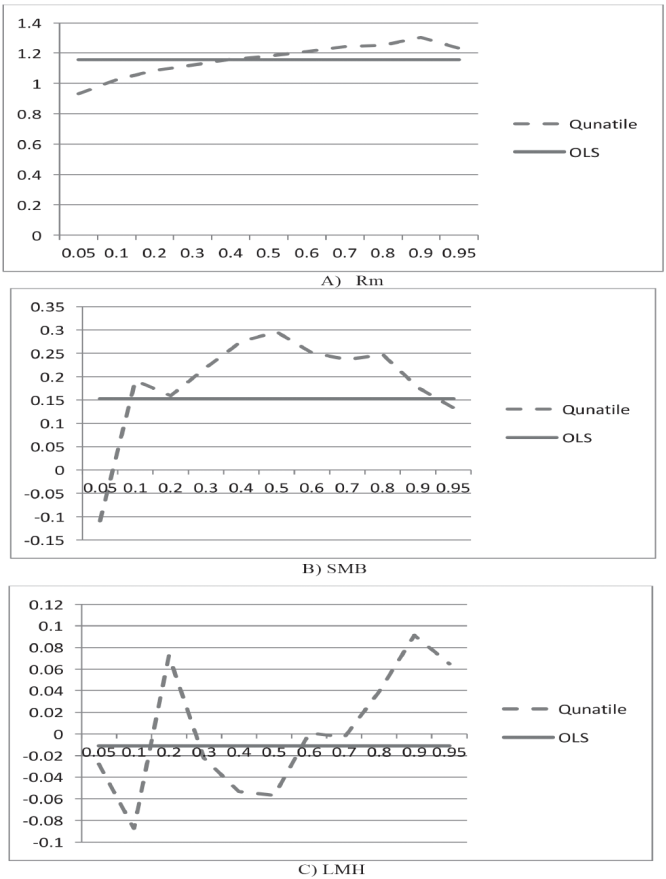
From the above Figure 2 it is clear that the value of the coefficient changes across the Quantile. The value of the coefficient changes rapidly in between the quartiles and with different frequency. For Rm the value of the coefficient increases with the higher Quantile. In case of SMB the coefficient value is negative in the lower Quantile and it becomes positive at the higher Quantile with difference in the frequencies across the Quantile. LMH coefficient value changes much more frequently across the quartile and is much more complicated. So, from the above graph it is clear that the OLS coefficient estimates only shows the average relationship between the portfolio returns and the risk variables. OLS analysis implies that the value of the coefficients is constant across the quintile which is really not the case as confirmed from the Figure 2. Further OLS coefficient estimates can only suggest the importance of the anomalies but unable to predict “Does LMH (value) influences portfolio returns differently for portfolios with low LMH than for average LMH?” Or “Does LMH (value) influences portfolio returns differently for portfolios with average LMH than for high LMH”? But on the other hand Quantile regression will state more comprehensive and clear picture of the effect of the predictors on the response variables as clearly shown in the above Figure 2. Hence, similar techniques can be replicated in other financial and economic studies where extensible factor model or OLS is used to reduce the error in study results.
Model prediction performance test
The study uses residual graphs for model performance test as shown in the Figure 3 below.
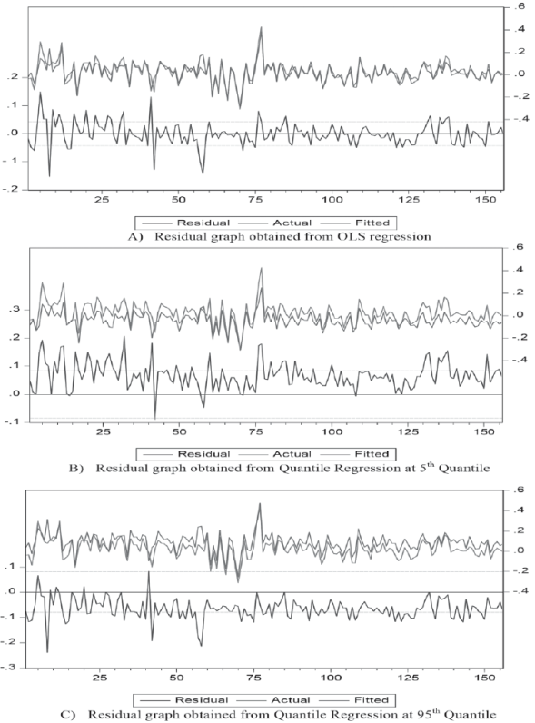
Figure 3 Residual graphs obtained from the OLS and Quantile regression (0.05 & 0.95) for portfolio 4
The residual graph shows the difference between the actual and fitted observation, value of zero or closer to zero is better. From above Figure 3 (A) residual graph of OLS regression high peaks are observed hence OLS unable to capture all the values effectively. From Figure 3 (B) & (C) Quantile regression both at 0.05 & 0.95 Quantile able to capture all the values as no peaks are observed. That justifies the supremacy of the Quantile regression over the OLS particularly in the end distributions.
Conclusion
The study starts with finding whether the 10 portfolios constructed from BSE 500 stocks based on P/B shows any value effect in return patterns. The study find there exist a very weak value effect in the return pattern of the P/B based portfolios. Further the study finds that the result estimated by Quantile regression is more comprehensive and robust as compared to OLS result. In many cases OLS shows positive/negative relationship between risk variables (Rm, SMB and LMH) and returns but the Quartile regression estimators shows it is not consistent across the Quantile. Hence, analyst or investment decision maker will get clearer picture about the risk return relationship and can avoid heavy loss. Residual graph confirms the best fit for Quantile regression result at the end tails. Hence, the study concludes that the Quantile regressions estimates are better and more comprehensive than the OLS estimates at the end distributions. The limitation of the study is that it is done in Indian context and hence in future one can test the same using global data with more factors.

