


 text in
  English (pdf)
 Article in xml format
 Article references
 Send this article by e-mail
 Cited by SciELO
  Similars in
SciELO
Similars in
SciELO 
 Permalink
Introduction
To understand the ecological dynamics and attributes of ecological communities, it is essential to estimate diversity accurately. Intertidal ecosystems are structurally complex environments and highly dynamic habitats (Daniel and Boyden 1975, Barreiros et al. 2004, Castellanos-Galindo et al. 2005). In intertidal rock pools, quantification of abundance and species richness is generally achieved with the application of invasive and non-invasive methods, like rock pool bailing and the use of chemicals to aid in the collection of fish (Gibson 1999, Wilding et al. 2001, Almada and Faria 2004, White and Brown 2013). Advantages of invasive methods include accurate and direct estimation of fish abundance and morphometric traits and the potential to collect specimens to analyze them in the laboratory. Invasive methods also provide more accurate identification at species level, especially when morphologically similar taxa or rare species occur in the sampling sites (Moring 1970, Griffiths 2005a, Malard et al. 2016).
Drawbacks of invasive methods include the disturbance and modification of habitat, stress exertion on individuals, potential behavioral changes of target organisms, and mortality and changes on the structure of assemblages of non-target organisms (Moring 1970, Almada and Faria 2004, Griffiths 2005a). The impact of invasive methods may be augmented by using a combination of methods such as bailing and chemicals that anesthetize target organisms, with undesired effects on research and conservation goals (Faria and Almada 1999, Almada and Faria 2004, Harasti et al. 2014). These impacts can be minimized by applying non-invasive techniques such as visual census or video recording (Gibson 1999, Wong et al. 2019). However, very little is known about the performance and trade-offs between invasive and non-invasive methods for sampling rock pool intertidal fishes.
Visual census has many desirable advantages when species that are threatened, endangered, or sensitive to handling occur in the study area (Wilding et al. 2001, Godinho and Lotufo 2010, Davis et al. 2018, Arndt and Fricke 2019). However, the visual census can be impacted by structural complexity in the habitat of study, observer biases (the researcher’s ability to identify and count individuals accurately), poor visibility, and fish response to the presence of the researcher (Brock 1982, Willis 2001, Galvan et al. 2009, Irigoyen et al. 2013, Bellwood et al. 2020). The general expectation is that visual census will underestimate abundance and richness, particularly for cryptic species (Brock 1982, Griffiths 2005b, Colton and Swearer 2010, Alzate et al. 2014). In open ecosystems, another less common drawback related to the visual census is the double counting of organisms that can cause abundance overestimation (Ward-Paige et al. 2010). In intertidal rock pools, the magnitude of double counting and other potential flaws during visual census is yet to be assessed.
In some instances, invasive methods have recorded higher values of fish abundance compared to visual census, but similar values of species richness (Griffiths 2005b). Although invasive and non-invasive sampling techniques could result in comparable abundances, species richness, or biodiversities, they do not quantify taxonomically distinct assemblages (Colton and Swearer 2010). These disparities between methods have been documented in many marine ecosystems (Brock 1982, Ackerman and Bellwood 2002, Colton and Swearer 2010, Bellwood et al. 2020) including intertidal rock pools (Davis et al. 2018).
Using different sampling techniques impedes comparing studies because there is no information to correct differences in estimates of abundance or species richness between methods (Castellanos-Galindo et al. 2014, González-Murcia et al. 2016, Andrades et al. 2018). To the best of our knowledge, there are no assessments comparing sampling techniques for the intertidal rock pool fishes in the Tropical Eastern Pacific.
Fish ethological traits can influence the performance of different sampling techniques (MacNeil et al. 2008, Colton and Swearer 2010). Species characteristics such as cryptic behavior, size of the individuals, coloration (camouflage, mimicry, and aposematic coloration), or solitary and schooling behavior increase biases in visual censuses (Brock 1982, Ackerman and Bellwood 2002, Colton and Swearer 2010). Furthermore, habitat variables such as rock pool volume and rugosity can interact and impact fish detection. Larger and structurally complex pools harbor more diverse fish assemblages than smaller rock pools (Mahon and Mahon 1994, Barreiros et al. 2004, Cunha et al. 2007, González-Murcia et al. 2020). Searching for species in larger and diverse habitats can, however, reduce detection or capture of fish and generate underestimation of abundance and species richness of fishes (Brock 1982, Willis 2001). To date, the influence of ethological traits, rock pool volume, and substratum rugosity on sampling methods for studying rock pool intertidal fish has not been well described. Understanding the flaws and strengths of sampling methods can aid with the detection of gaps in research to be addressed in subsequent studies for intertidal fishes.
The complex dynamic in intertidal systems usually requires the application of different sampling techniques at the expense of weakening quantitative comparisons. Determining the consistency of different methods to obtain fundamental ecological metrics such as abundance, species richness, and diversity is of interest for conservation and research purposes. Our goal was to compare abundance, species richness, and assemblage structure of rock pool intertidal fishes obtained with bailing and visual census sampling methods. In addition, we aimed to examine the impact of fish behavior, rock pool volume, and rock pool substratum rugosity on the detection of fishes with the 2 methods. We predicted that we would detect higher abundances and species richness with rock pool bailing than with the visual census and that those assemblages recorded with the visual census would differ from those recorded with the bailing method. We expected differences in fish detection between methods would be associated with fish behavior. Moreover, we expected that rock pool volume and substratum rugosity would negatively affect the performance of both sampling methods and that their effects were going to be exacerbated in the visual census.
Materials and methods
Study area and sampling design
El Zonte is an area with multiple small rocky shores located in Chiltiupán, La Libertad, El Salvador. Semidiurnal tides ranged from -20 to 230 cm (MARN 2018); the tide calendar and total time of rock pool emersion during low tide were used to estimate the intertidal heights of 10 randomly selected rock pools (Fig. 1). The elevation of rock pools above the low tide line was 43-96 cm. Sampling (sampling period) was conducted 13 times across the complete set of 10 rockpools from June to December 2018. Each pool was sampled using a visual census and then the bailing method. A sampling event was defined as the process of conducting both methods in a single rock pool. For the visual census, the observer approached a rock pool, surveyed it for 15 minutes, and recorded the number of individuals per species. The bailing method was performed with an electric underwater bilge pump with a 12v battery and maximum capacity of 3,700 gallons per hour (~17 m3) (Griffiths 2003a, b; González-Murcia et al. 2016; Wong et al. 2019; González-Murcia et al. 2020), and with hoses and buckets to bail out water manually and accelerate the process. Both methods were conducted following the same protocol even when fish were not detected in visual census to discard false negatives and contrast the correspondence of methods. Visual census always preceded rock pool bailing sampling, and sampling methods (treatments) were not randomly allocated since the bailing method is invasive and can have detrimental impacts on fish, which influences the outcomes of the visual census. Crevices and spaces under rocks and fleshy algae were searched to capture the fish. Fish were identified, kept in buckets, and returned to the rock pools after sampling. The same rock pools were sampled the 2 following days with both methods. For each sampling campaign, some specimens were collected and deposited at the Museo de Historia Natural de El Salvador (MUHNES) collection under catalogue numbers from MUHNES 40-1034 to 40-1054 (Table S1). Sampling was conducted only once in June and twice a month from July to December 2018.
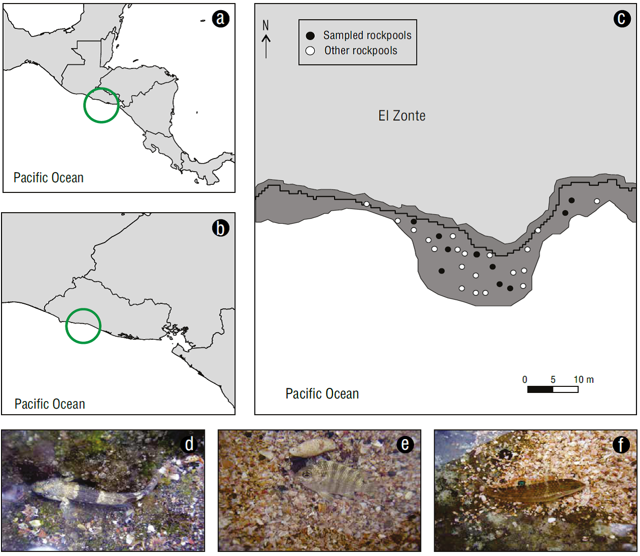
Figure 1 Rock pools sampling area in Central America (a), El Salvador (b), El Zonte, La Libertad (c), with examples of residents, Bathygobius ramosus (d); opportunist, Abudefduf concolor (e); and transients, Halichoeres sp. (f) species. Image credits: Saúl González-Murcia.
Each fish species was classified according to their rock pool use. The residency categories were the following: permanent residents, opportunists, and transients (Griffiths 2003a, b). Similarly, according to their behavioral affinities, each species was categorized as solitary, aggregating, cryptic, and territorial (Griffiths 2003a, b). Residency categories and behavioral affinities interrelate because permanent residents tend to be solitary and cryptic (Gibson and Yoshiyama 1999, White and Brown 2013). Likewise, opportunists aggregate in schools or are solitary and swim in the water column near the surface, whereas transients can display any type of behavioral affinity. To compare how fish behavior could impact fish detection between methods, rock pool residency categories were used; this classification has mutually exclusive categories and was considered a better proxy for fish detection by sampling method (see data analyses).
Rock pool physical attributes, structural traits, and substratum rugosity
Before collecting the fish, for each rock pool, we obtained 3 measurements of width (W), length (L), depth (D), and one of the perimeter (P). Volume was estimated with the following formula:
where V is the rock pool volume; SA, the surface area of the rock pool, estimated with the average width (W) and length (L) [SA = W × L]; and D is the average rock pool depth. Rock pool volume ranged from 0.01 m3 to 2.79 m3 (Table 1). Rock pool substratum rugosity was calculated by dividing the linear distance (LD) between 2 points of the rock pool by the length of the contoured surface profile (RD) between the same 2 points. We used the following formula to generate a percentage that indicated low (0%) to high (100%) rock pool substratum rugosity (Table 1):
Table 1 Metrics of depth (m), width (m), length (m), surface area (m2), volume (m3), substratum rugosity (%), and intertidal height location (m) measured in 10 intertidal rock pools. Standard error (SE). The volume was estimated using the following formula: V = SA × D; where SA is the surface area of the rock pool (W × L) estimated with the average width (W) and length (L), and D is the average rock pool depth; there are no SE for volume values.
| Pool | Depth (m) ± SE | Width (m) ± SE | Length (m) ± SE | Surface area (m2) | Volume (m3) | Substratum rugosity (%) | Height (m) |
| 1 | 0.26 ± 0.17 | 0.73 ± 0.05 | 1.30 ± 0.17 | 0.95 | 0.25 | 1 | 0.96 |
| 2 | 0.23 ± 0.07 | 0.52 ± 0.05 | 0.79 ± 0.04 | 0.41 | 0.10 | 9 | 0.94 |
| 3 | 0.73 ± 0.16 | 2.12 ± 0.54 | 1.81 ± 0.39 | 3.84 | 2.79 | 5 | 0.54 |
| 4 | 0.50 ± 0.02 | 0.57 ± 0.11 | 0.88 ± 0.09 | 0.50 | 0.25 | 9 | 0.66 |
| 5 | 0.28 ± 0.08 | 1.80 ± 0.54 | 2.98 ± 0.52 | 5.35 | 1.52 | 1 | 0.43 |
| 6 | 0.18 ± 0.13 | 1.57 ± 0.36 | 1.3.7 ± 0.11 | 2.16 | 0.38 | 19 | 0.74 |
| 7 | 0.08 ± 0.02 | 0.08 ± 0.05 | 1.30 ± 0.24 | 0.60 | 0.05 | 0 | 0.74 |
| 8 | 0.65 ± 0.03 | 0.65 ± 0.03 | 0.78 ± 0.10 | 0.33 | 0.22 | 15 | 0.43 |
| 9 | 0.06 ± 0.02 | 0.45 ± 0.05 | 0.55 ± 0.05 | 0.25 | 0.01 | 7 | 0.96 |
| 10 | 0.07 ± 0.03 | 0.17 ± 0.08 | 0.79 ± 0.15 | 0.14 | 0.01 | 9 | 0.89 |
Data analysis
Differences in abundance and species richness of fishes between methods were analyzed using multilevel models based on a Bayesian approach (McElreath 2016) with the rstan package (Stan Development Team 2020). The models included fish abundance as a response variable and the population effects of sampling method, fish residency category (proxy of behavior affinities), rock pool volume, and percentage of rugosity plus the interaction between sampling method and fish residency category. Varying effects of the rock pool ID (1-10) and sampling period (1-13) were also included to account for the dependency structures imposed by the hierarchical design. The models were fitted using a negative binomial distribution to account for overdispersion. Markov chain Monte Carlo (MCMC) sampler was run for 5 chains and 20,000 iterations per chain and a warmup of 2,000 for each chain. Thinning was set to 8, and the priors for the intercept were set to normal (0,10) and slope normal (0,1). Priors for the varying effect were set to (0,1) and the dispersion parameter was (0.01,0.01). The MCMC diagnostics suggested that, for each model, the chains were well mixed and converged on a stable posterior (all Rhat values < 1.05). Residuals patterns were tested for normality, dispersion, and variance with the DHARMa package (Hartig 2021). To contrasts levels of explanatory variables, intervals of the highest probability compatibility intervals (HPCI) were used as measurements of uncertainty. The Exceedance P value was used as a metric for the occurrence of a given event and represents the probability that a certain value will be exceeded in a predefined situation (McElreath 2016). Rock pool volumes of 0.1 m3, 0.5 m3, 1.5 m3, and 2.5 m3 and substratum rugosity (%) values of 1%, 10%, and 19% were used as benchmarks to contrast the trends in abundance and species richness estimated with the models. Models for subsets of resident, opportunists, and transient fish were constructed using the sampling method, volume, and rugosity as population effects and the rock pool ID (1-10) and sampling period (1-13) as varying effects to determine changes in detection for each group (Table S2-S7).
Changes in assemblage structure and taxonomic distinctiveness related to sampling methods were assessed using a non-metric multidimensional scaling (NMDS) analysis (Quinn and Keough 2002). Abundance of fish species were square root transformed and used to generate a matrix of dissimilarities calculated with the Bray-Curtis distance measure. A “dummy species variable” that contained the value 1 was incorporated to reduce difficulties in the estimation of distance (Clarke et al. 2006). The NMDS was constructed using the monoMDS function (nonmetric multidimensional scaling with stable solution from Random starts, axis scaling, and species scores) setting the number of starts to 999 runs and basing the stress on monotonic (non-linear) regression. The correspondence between the ordination distances and observed dissimilarity was assessed via diagnostic plots of stress, goodness of fit tests, and R-squared. These analyses were performed with the Vegan package (Oksanen et al. 2022).
Differences in the structure of fish assemblages detected between sampling methods were tested with the permutational multivariate analysis of variance using the Adonis function that generates an R 2 value (effect size), which represents the percentage of variation explained by the supplied category, and a P value, which determines the statistical significance (Oksanen et al. 2022). The correlation of the species with the sampling methods was obtained with the envfit function considering only species with P < 0.05 (R Core Team 2019). In addition, the contribution of species to the differences detected between sampling methods was tested via indicator species analyses (De Cáceres et al. 2010). For the analysis, the sampling method was set as classification criteria to compare the observed patterns of species distribution. The phi correlation coefficient was corrected for unequal group sizes generating a r.g value. We selected the influential fish species with values of r.g > 0.6 and P < 0.05 (De Cáceres and Legendre 2009). All the analyses were conducted in the statistical program R (R Core Team 2019).
Results
General patterns in fish assemblages between sampling methods
We detected more individuals and species with the rock pool bailing method compared to the visual census method (Fig. 2). We detected a total of 1,749 individuals of 14 species with the rock pool bailing and 438 individuals of 8 species with the visual census. In total, the bailing method detected almost 4 times the number of fish and 2 times the number of species detected with the visual census method. The abundance obtained per species with the rock pool bailing method was higher than the abundance recorded using the visual census for all the species except for Mugil curema Valenciennes, 1836 (Fig. 2). The 6 additional species detected with the rock pool bailing method, which were undetected with the visual census (Gobiesox daedaleus Briggs, 1951; Ophioblennius steindachneri Jordan and Evermann, 1898; Paraclinus beebei, Hubbs 1952; Paraclinus monophthalmus [Günther, 1861], Rypticus nigripinnis Gill, 1861; and Tomicodon sp1 Brisout de Barneville, 1846), are resident species with cryptic behavior. The rock pool bailing method not only detected higher fish abundance and more species than the visual census method, but also corrected erroneous records of absence (false negatives) of fish in the rock pools obtained with the visual census when fish were subsequently detected with the bailing method. False negatives were recorded with the visual census in 32 sampling events in different sampling periods and rock pools, between June and December for the 10 sampled rock pools.
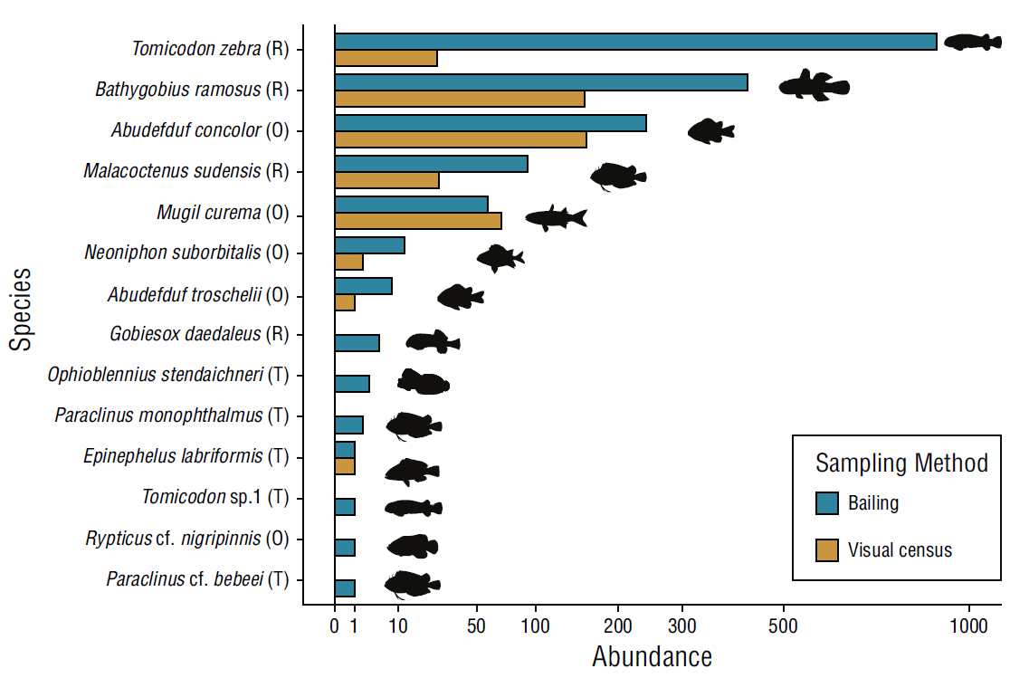
Figure 2 Total abundance by fish species recorded using bailing and visual census in rock pools of El Zonte, 2018. The scale on the X axis has been square root transformed to display abundance values between 0 and 100 and abundances larger than 100. Letters next to species names refer to residency categories: (R) resident, (O) opportunist, (T) transient.
Fish abundance between the sampling methods, fish residency categories, rock pool volume, and substratum rugosity
The sampling method, residency categories, rock pool volume, and rugosity collectively explained 67% (R 2 = 0.67) of the variability in fish abundance (Table 2). Rock pool ID and sampling period explained 6% and 4% of the variability, respectively. The model that included rock pool ID and sampling period covariates attained 77% of the variability in abundance. Higher abundances of resident (Exceedance P = 1.00), opportunist (Exceedance P = 0.98), and transient (Exceedance P = 0.99) fish were detected with the bailing method compared with those detected with the visual census method (Tables 3, 4). The rock pool bailing method detected almost 4 times the number of resident fishes, 1.5 times the opportunist fish, and almost 8 times the transient individuals compared with the visual census method (Table 4; Fig. 3a). Despite higher abundances detected with rock pool bailing, statistical differences were not reached for opportunist and transient fish (Table 4).
Table 2 Fish abundance associated to sampling method, residency category, rock pool water volume, rugosity, and varying effects of the sampling event and rock pool ID for all the species (R 2 = 67%). Mean abundance calculated with the model (Estimate), standard error (SE), 95% highest probability compatibility intervals (HPCI); evidence of autocorrelation during the generation of the posterior (Rhat) and the values of Ȓ ≤ 1.05 indicate low chances of autocorrelation in the sampling of the ESS, where ESS is the effective sample size, which is a metric to measure the amount by which autocorrelation in samples increases uncertainty in comparison to an independent sample.
| Term | Estimate | SE | Lower HPCI | Upper HPCI | Rhat | ESS |
| Intercept | 1.510 | 0.14 | 1.220 | 1.770 | 0.99 | 10,696 |
| Visual census | -1.580 | 0.17 | -1.930 | -1.230 | 1 | 11,396 |
| Opportunist | -1.450 | 0.18 | -1.810 | -1.100 | 1 | 10,585 |
| Transient | -4.740 | 0.33 | -5.400 | -4.100 | 1 | 11,675 |
| Volume | 0.086 | 0.01 | 0.060 | 0.120 | 1 | 11,049 |
| Rugosity | -0.070 | 0.02 | -0.126 | -0.025 | 0.99 | 11,069 |
| Visual census: opportunist | 1.150 | 0.25 | 0.661 | 1.650 | 0.99 | 11,000 |
| Visual census: transient | -0.590 | 0.68 | -2.020 | 0.664 | 0.99 | 11,205 |
| Reciprocal dispersion | 0.870 | 0.11 | 0.650 | 1.090 | 0.99 | 10,212 |
| Sigma rock pools: sampling event | 0.460 | 0.40 | 0 | 1.190 | 1 | 1,738 |
| Sigma rock pools identity | 0.470 | 0.40 | 0 | 1.190 | 1 | 1,797 |
| Mean_PPD | 2.890 | 0.47 | 2.070 | 3.870 | 0.99 | 11,281 |
| Log-posterior | 0.001 | 15.39 | 0.001 | -0.003 | 0.99 | 10,023 |
Table 3 Mean fish abundance by method and residency categories. 95% Highest Probability Compatibility Intervals (HPCI). Whenever the ranges of the HPCI between categories do not overlap, significant differences in abundance are supported.
| Sampling method and residency category | Estimate | Lower HPCI | Upper HPCI |
| Bailing and resident | 4.5000 | 3.3000 | 5.8800 |
| Visual census and resident | 0.9200 | 0.6300 | 1.2600 |
| Bailing and opportunist | 1.0400 | 0.7100 | 1.4400 |
| Visual census and opportunist | 0.6800 | 0.4700 | 0.9600 |
| Bailing and transient | 0.0300 | 0.0100 | 0.0600 |
| Visual census and transient | 0.0040 | 0.0004 | 0.0100 |
Table 4 Contrast of fish abundance of different residency categories captured using the bailing and visual census methods. Contrasts between levels of explanatory variables using the 95% confidence intervals of the highest probability compatibility intervals (HPCI) and exceedance P value, which is the probability that a certain value will be exceeded in a predefined situation and represents a metric for the occurrence of a given event.
| Sampling method and residency category | Estimate | Lower HPCI | Upper HPCI | Exceedance P |
| Bailing and resident/visual census and resident | 4.850 | 3.307 | 6.75 | 1 |
| Bailing and opportunist/visual census and opportunist | 1.526 | 0.998 | 2.12 | 0.988 |
| Bailing and transient/visual census and transient | 8.764 | 1.446 | 28.93 | 0.990 |
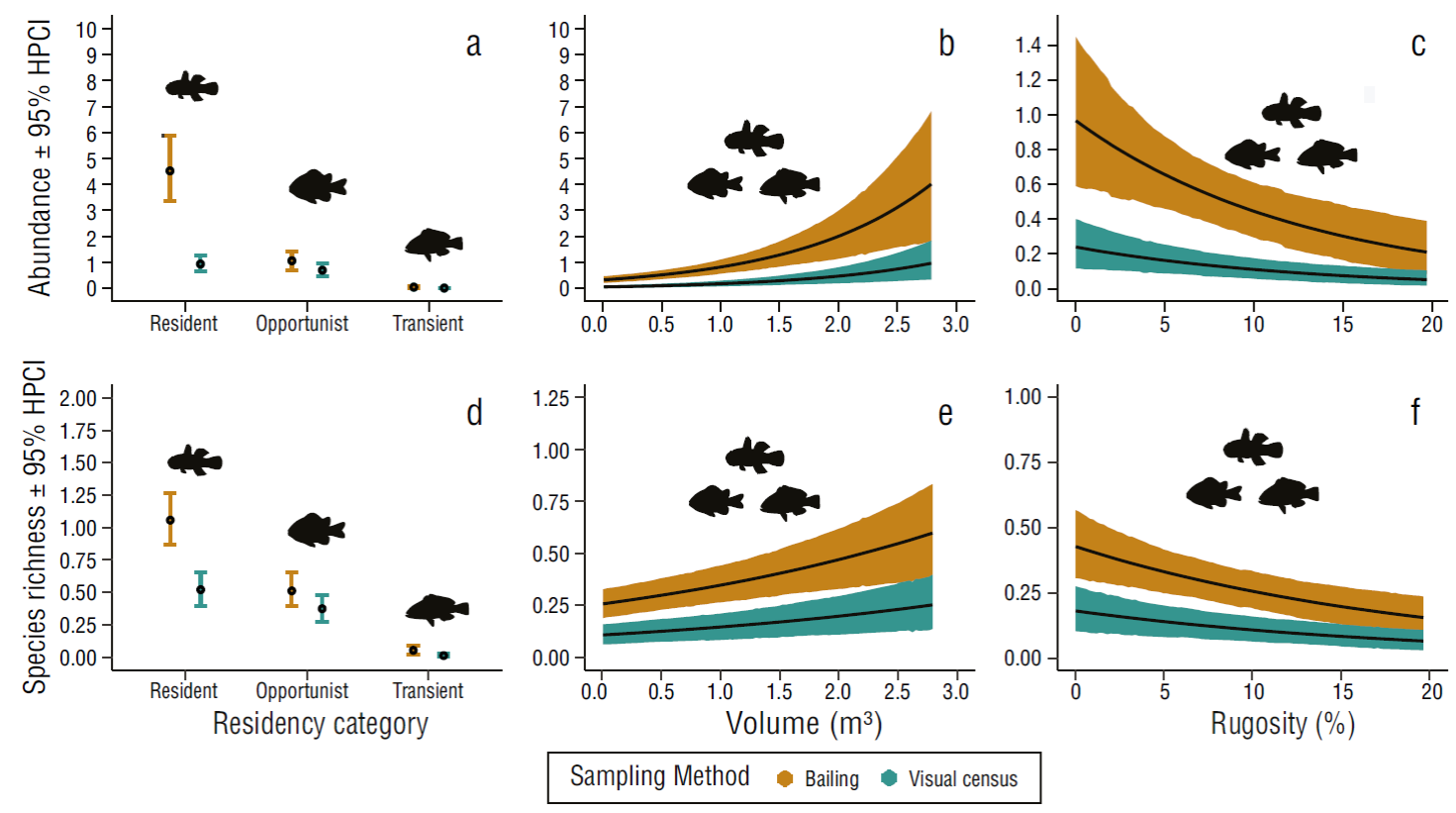
Figure 3 Average abundance and species richness of fish by residency category (see Materials and Methods) (a, d), rock pool volume (b, e), and rock pool substratum rugosity recorded using the bailing and visual census methods in rock pools of El Zonte, 2018 (c, f). Whiskers and shaded areas represent 95% confidence intervals of the highest probability compatibility intervals (HPCI).
Rock pool volume was positively associated with higher fish abundance with both detection methods. On average, the bailing method detected more fish than the visual census when rock pool volume increased (Fig. 3b). Differences in fish abundance detected between sampling methods were more evident in larger pools where more fish were detected with the bailing method (Table 5). The impact of rock pool volume on fish detection between the 2 sampling methods remained evident across all fish residency categories. Rock pool bailing consistently detected ~4 times more resident, ~1.5 times more opportunist, and ~3 times more transient fish in all rock pool volumes (from 0.01 m3 to 2.79 m3) compared to the visual census (Tables S2, S3).
Table 5 Mean fish abundance detected by method, volume for rock pools of 0.1, 0.5, 1.5, and 2.5 m3, and substratum rugosity values of 1%, 10%, and 19%. 95% Highest probability compatibility intervals (HPCI). Whenever the ranges of the HPCI between categories do not overlap, significant differences in abundance are supported.
| Contrast | Estimate | Lower HPCI | Upper HPCI |
| Volume and method | |||
| Volume 0.1 m3 | |||
| Bailing | 0.39 | 0.27 | 0.54 |
| Visual census | 0.09 | 0.05 | 0.15 |
| Volume 0.5 m3 | |||
| Bailing | 0.55 | 0.40 | 0.74 |
| Visual census | 0.13 | 0.07 | 0.20 |
| Volume 1.5 m3 | |||
| Bailing | 1.37 | 0.91 | 1.93 |
| Visual census | 0.33 | 0.17 | 0.54 |
| Volume 2.5 m3 | |||
| Bailing | 3.37 | 1.71 | 5.51 |
| Visual census | 0.77 | 0.31 | 1.38 |
| Rugosity and method | |||
| Rugosity 1% | |||
| Bailing | 0.87 | 0.56 | 1.27 |
| Visual census | 0.21 | 0.11 | 0.35 |
| Rugosity 10% | |||
| Bailing | 0.43 | 0.29 | 0.60 |
| Visual census | 0.10 | 0.05 | 0.17 |
| Rugosity 19% | |||
| Bailing | 0.20 | 0.08 | 0.39 |
| Visual census | 0.05 | 0.01 | 0.10 |
Fish detection decreased with the increase of substratum rugosity for both methods (Fig. 3c). In rock pools with low levels of substratum rugosity (1%), the bailing method detected ~1 species on average, but the chances of detecting at least one individual decreased drastically in areas with higher complexity (19% ~0.43). The visual census method performed poorly on areas with low substratum rugosity (1%) and fish detection declined abruptly in pools with 20% rugosity (Table 5). The reduction in fish detection due to substratum rugosity was associated with fish residency categories. In rock pools with low (1%) to high rugosity (19%) rock pool bailing sampling detected ~4 times more resident, ~1.5 times more opportunist, and ~3 times more transient fish compared to the visual census (Tables S2, S4).
Fish species richness between sampling methods, residency categories, rock pool volume, and substratum rugosity
The sampling method, fish behavior, rock pool volume, and rugosity influence the detection of fish species and collectively explained 64% (R 2 = 0.64) of the variability in species richness (Table 6). Rock pool ID and sampling period explained 4.8% and 3.6% of the variability in fish species richness, respectively. When the variables rock pool and sampling period were included in the model, a total of 72% of the variability in species richness was explained. The bailing method detected more resident (P = 1.00), opportunist (P = 0.95), and transient (P = 99) fish species than the visual census method (Fig. 3d). Likewise, the rock pool bailing method detected on average almost double the species of resident fish, 1.37 times more opportunist species, and almost 5 times more transient species than visual census (Fig. 3d) (Tables 5-9). However, statistically significant differences in fish detection between sampling methods were not observed for opportunist and transient species.
Table 6 Fish species richness associated with the sampling method, residency category, rock pool water volume, rugosity, and varying effects of sampling event and rock pool ID for all the species. Mean abundance calculated with the model (Estimate), standard error (SE), 95% highest probability compatibility intervals (HPCI), evidence of autocorrelation during the generation of the posterior (Rhat), and the values of Ȓ ≤ 1.05 indicate low chances of autocorrelation in the sampling of the effective sample size (ESS); ESS is a metric to measure the amount by which autocorrelation in samples increases uncertainty in comparison to an independent sample.
| Term | Estimate | SE | Lower HPCI | Upper HPCI | Rhat | ESS |
| Intercept | 0.0545 | 0.0900 | -0.1338 | 0.2440 | 0.99 | 11,151 |
| Visual census | -0.7091 | 0.1446 | -0.9959 | -0.4307 | 0.99 | 11,494 |
| Opportunist | -0.7240 | 0.1453 | -1.0148 | -0.4493 | 0.99 | 11,196 |
| Transient | -3.0030 | 0.3324 | -3.6718 | -2.3800 | 0.99 | 11,298 |
| Volume | 0.0342 | 0.0067 | 0.0170 | 0.0433 | 1 | 10,886 |
| Rugosity | -0.0517 | 0.0149 | -0.0800 | -0.0214 | 1 | 11,102 |
| Visual census: opportunist | 0.3899 | 0.2256 | -0.0406 | 0.8434 | 0.99 | 11,234 |
| Visual census: transient | -0.8329 | 0.6476 | -2.1050 | 0.3985 | 0.99 | 10,867 |
| Reciprocal dispersion | 7.5500 | 1.9700 | 4.3700 | 11.7500 | 0.99 | 10,825 |
| Sigma rock pools: sampling event | 0.0478 | 0.0620 | 0.04 × 10⁻⁷ | 0.1843 | 0.99 | 8,535 |
| Sigma rock pools identity | 0.0450 | 0.0622 | 0. 01 × 10-7 | 0.1857 | 0.99 | 9,468 |
| Mean_PPD | 0.4890 | 0.0379 | 0.4172 | 0.5635 | 1 | 10,949 |
| Log-posterior | -936.9909 | 14.4208 | -936.617 | -908.67267 | 1.000018 | 10,978 |
Table 7 Mean fish species richness by method and residency categories. 95% Highest probability compatibility intervals (HPCI). Whenever the ranges of the HPCI between categories do not overlap, significant differences in abundance are supported.
| Sampling method and residency category | Estimate | Lower HPCI | Upper HPCI |
| Bailing and resident | 1.0561 | 0.8567 | 1.2536 |
| Visual census and resident | 0.5196 | 0.3949 | 0.6507 |
| Bailing and opportunist | 0.5120 | 0.3909 | 0.6447 |
| Visual census and opportunist | 0.3709 | 0.2683 | 0.4790 |
| Bailing and transient | 0.0525 | 0.0235 | 0.0904 |
| Visual census and transient | 0.0112 | 0.0013 | 0.0281 |
Table 8 Contrast of fish species richness of different residency categories captured using the bailing and visual census methods. Contrasts between levels of explanatory variables using the 95% confidence intervals of the highest probability compatibility intervals (HPCI) and Exceedance P value, which is the probability that a certain value will be exceeded in a predefined situation; this was used as metric for the occurrence of a given event.
| Sampling method and residency category | Estimate | Lower HPCI | Upper HPCI | Exceedance P |
| Bailing and resident/visual census and resident | 2.03 | 1.501 | 2.66 | 1 |
| Bailing and opportunist/visual census and opportunist | 1.38 | 0.936 | 1.92 | 0.96 |
| Bailing and transient/visual census and transient | 4.67 | 0.968 | 14.70 | 0.99 |
Table 9 Mean fish species richness detected by method, volume for rock pools of 0.1 m3, 0.5 m3, 1.5 m3, and 2.5 m3 and substratum rugosity values of 1%, 10%, and 19%. 95% Highest probability compatibility intervals (HPCI). Whenever the ranges of the HPCI between categories do not overlap, significant differences in abundance are supported.
| Contrast | Estimate | Lower HPCI | Upper HPCI |
| Sampling method | |||
| Bailing | 0.57 | 0.48 | 0.65 |
| Visual census | 0.32 | 0.26 | 0.38 |
| Volume and method | |||
| Volume 0.1 m3 | |||
| Bailing | 0.48 | 0.39 | 0.57 |
| Visual census | 0.27 | 0.21 | 0.33 |
| Volume 0.5 m3 | |||
| Bailing | 0.54 | 0.46 | 0.63 |
| Visual census | 0.30 | 0.24 | 0.36 |
| Volume 1.5 m3 | |||
| Bailing | 0.73 | 0.59 | 0.87 |
| Visual census | 0.41 | 0.32 | 0.50 |
| Volume 2.5 m3 | |||
| Bailing | 0.98 | 0.72 | 1.27 |
| Visual census | 0.55 | 0.39 | 0.73 |
| Rugosity and method | |||
| Rugosity 1% | |||
| Bailing | 0.77 | 0.62 | 0.92 |
| Visual census | 0.43 | 0.34 | 0.53 |
| Rugosity 10% | |||
| Bailing | 0.48 | 0.40 | 0.57 |
| Visual census | 0.27 | 0.21 | 0.33 |
| Rugosity 19% | |||
| Bailing | 0.30 | 0.19 | 0.42 |
| Visual census | 0.17 | 0.11 | 0.24 |
The bailing and visual methods detected more fish species in larger pools. On average, the bailing method detected more species than the visual census when rock pool volume increased (Fig. 3e). These differences were more evident in larger pools where more fish were detected with the bailing method than with visual census. In rock pools of 0.5 m3 volume or less, the difference in detection of fishes between methods was small, but in rock pools of 2.5 m3 volume, the bailing method detected ~2 fish species compared to ~1 species detected with the visual census (Fig. 3e, Table 9). General trends in species detection associated with volume were sustained across fish residency categories. The rock pool bailing method detected ~2 more resident species, ~1.3 more opportunist species, and ~3 more transient species than the visual census method (Table S5, S6).
The number of species detected with the bailing and visual census methods decreased when substratum rugosity increased. However, the bailing method consistently detected fish species more effectively than the visual census. In rock pools with rugosity values of 5%, detection of fish species was ~2 times higher with the bailing method than with visual census. This trend was consistent, and in rock pools of 19% rugosity, fish species detection was almost ~0.66 times lower for both methods. Nevertheless, rock pool bailing still performed better than visual census (Fig. 3f, Table 9). The decline in fish species regarding substratum rugosity was also associated with residency categories. Rock pool bailing detected ~2 more resident species, ~1.3 more opportunist, and ~3 more transient species compared to the visual census method (Table S5, S7).
Fish assemblage structure and taxonomic composition detected between sampling methods
Fish assemblages recorded with the bailing and visual census methods yielded different community compositions (Fig. 4, Adonis = 9.0476, d.f. = 1, P < 0.001). Visual census detected fish assemblages with similar contribution of resident and opportunist species. On the other hand, the bailing method detected fish assemblages with higher contributions of resident species that dominated in terms of abundance (Fig. 4). The species that characterized the assemblages were the resident species Bathygobius ramosus (r 2 = 0.61, P < 0.01), Tomicodon zebra (r.g = 0.61, P < 0.01), and Malacoctenus sudensis (r 2 = 0.34, P < 0.01), which were detected in higher abundances with the bailing method, and the opportunist species Abudefduf concolor (r 2 = 0.28, P < 0.01) and M. curema (r 2 = 0.55, P < 0.01), which were equally detected with the visual census and bailing methods. The indicator species analysis detected that the resident species B. ramosus (r.g = 0.17, P < 0.05) and T. zebra (r.g = 0.20, P < 0.01) were typical species that appear to have been detected mainly by the rock pool bailing method.
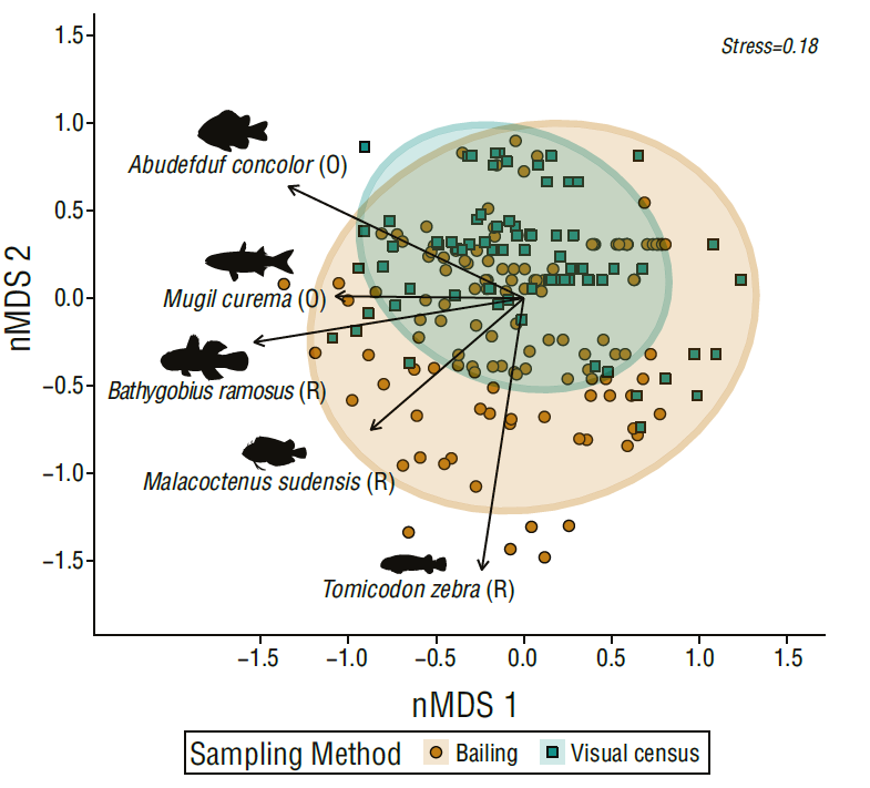
Figure 4 Fish assemblages detected with bailing and visual census in 10 rock pools sampled 13 times between June and December 2018 in El Zonte, El Salvador, based on a non-metric dimensional scaling (nMDS). Total abundance data were square root transformed, and dissimilarities are based on a Bray-Curtis similarity index metric, ellipses display 95% confidence intervals. Residents (R), opportunists fish species (O).
Discussion
The sampling methods showed different estimates of abundance, species richness, and composition and structure of assemblages. The bailing method consistently detected more fish species and individuals than visual census. The visual census method largely underestimated fish abundance and species richness, and detected 75% fewer fish individuals and 40% fewer species compared to the rock pool bailing method. The visual census has been disfavored as a sampling method since it has consistently underestimated abundance and species richness (Christensen and Winterbottom 1981, Brock 1982, Ackerman and Bellwood 2000, Alzate et al. 2014). The magnitude of the differences indicates that 50% of individuals and 40% of species are overlooked even with the most exhaustive visual census methods (Ackerman and Bellwood 2000). Griffiths (2005b) detected differences with larger magnitudes in rock pool systems, with the visual census showing 80-87% less abundance and 50-66% lower species richness than rock pool bailing, as did Wong et al. (2019) with 70% lower abundance and 33% fewer species detected with the visual census. These deficiencies of the visual census method call for a reconsideration of applying visual census when sampling intertidal rock pool fishes.
Visual census frequently failed to detect fish that were subsequently recorded during rock pool bailing, which recorded a false negative result for visual census (recording absences when fish were present). However, the bailing method was not infallible; in very few cases, fish, such as M. curema, were detected during visual census but were not detected with the bailing method. This could be due to fish retreating and hiding in crevices during the bailing of rock pools. In some cases, fish stay hidden or get trapped in crevices when the pool is being bailed and their detection or capture is unsuccessful. Alternatively, this result can represent potential double counting bias since M. curema tends to form schools, and using visual census on this species might overestimate abundance (Ward-Paige et al. 2010). Despite these drawbacks, fish detection was higher with the rock pool bailing method compared to the visual census method; therefore, the rock pool bailing method is a more accurate technique to assess intertidal fish.
The rock pool bailing method detected almost 4 times more resident fish than the visual census method. With the visual census, resident fish were constantly underrepresented in all levels of rock pool volume and substratum rugosity. The inconsistencies in detection of fishes between methods also generated discrepancies in the assemblages recorded between both methods. The similar contribution of resident and opportunist species in assemblages described with the visual census evidenced the weaknesses of resident species detection with this method. Fish behavior can affect sampling detectability, and our results support that visual census were biased towards opportunist species that frequently show traits that can be easily observed. Ethological traits are the most influential factors in fish detection during the visual census method (MacNeil et al. 2008, Colton and Swearer 2010), and resident fishes in intertidal systems are not an exception.
The detection of cryptic species has been the weakness of sampling methods in marine environments (Brock 1982, Ackerman and Bellwood 2000, Godinho and Lotufo 2010, Davis et al. 2018). Nocturnal species are not only inactive, but also hidden during diurnal visual census, causing a steep decline in the probability of their detection specially when using the visual census method. The differences between the bailing and visual census methods were less marked for opportunist and transient fishes. Thus, visual census could be suitable to study and quantify fish diversity for diurnally active opportunist and transient species and could potentially be applied as a complementary technique instead of a stand-alone method. However, the use of the visual census in rock pool habitats should be conducted with caution, as our results coincide with previous findings (Christensen and Winterbottom 1981, Griffiths 2005a, Wong et al. 2019); visual census estimates were inaccurate, biased towards opportunist and transient fishes, and less reliable than the rock pool bailing method.
Both methods detected less species and individuals in rock pools with higher rugosity, but samplings with the bailing method constantly yielded better results than the visual census method. The extent to which rugosity affects fish detection can be linked to fish behavior, as cryptic resident fish might retreat in burrows when observers are present and during the bailing process, whereas opportunist and transients are less likely to hide in burrows than residents. Changes in rugosity provide more refuges and microhabitats that can sustain higher abundances and more fish species (Davis 2000, Griffiths et al. 2006, González-Murcia et al. 2020). Unfortunately for sampling purposes, substratum rugosity reduces sampling accuracy because areas of high substratum rugosity provide greater shelter mostly for cryptic fishes, which compromises the detection of individuals (Brock 1982). In some systems, severe underestimations of up to 82% less species richness and 73% abundance have been attributed to habitat complexity (Willis 2001). Furthermore, higher habitat complexity can increase the likelihood that species will be erroneously identified, counted, and quantified and that target species estimation will be affected (Brock 1982).
Rock pool bailing alone appears to be effective enough for sampling intertidal fishes reducing the bias towards opportunist and transient species. This method offers many advantages and provides opportunities to collect more information from target species. Ichthyocides can be used, but they may have detrimental impacts on enclosed systems such as rock pools. Visual census underrates abundance and species richness and produces inaccurate estimations; however, it may need to be used whenever other sampling methods are not suitable. Visual census can also overlook large individuals of secretive species and underrepresent size classes in rock pool fishes (Griffiths 2005a, Griffiths et al. 2006). Consequently, data from visual census in intertidal rock pool fishes should be analyzed cautiously.
El Zonte is an area with low intertidal fish diversity (González-Murcia et al. 2020), whereas other intertidal areas have higher abundance and species richness of resident, opportunist, and transient species (González-Murcia et al. 2012, González-Murcia et al. 2016). We suspect that the inaccuracies of using the visual census in intertidal areas with higher diversity would be magnified. Emerging technologies can ameliorate or supplement the accuracy of visual census (Colton and Swearer 2010, Dorman et al. 2012, Harasti et al. 2015, Davis et al. 2018). Alternative techniques are not free from the drawbacks of the visual census (Colton and Swearer 2010, Davis et al. 2018). The efficacy of these methods in intertidal areas of the Tropical Eastern Pacific needs to be assessed and validated. Modelling functions have been used to correct inequalities between sampling methods (Christensen and Winterbottom 1981). Due to the high variability within intertidal systems, we consider that modelling, extrapolation, and prediction of abundance and species occurrence must be conducted with prudence.
In conclusion, we contrasted the rock pool bailing and visual census methods with respect to how accurately these detect intertidal rock pool fishes with different residency categories under different levels of rock pool volume and substratum rugosity. The bailing method yielded higher abundances and species richness in pools of different volumes and rugosity levels compared to visual census. The rock pool bailing method reduced the rate of false negatives as it accurately detected fish that were not detected with the visual census. Resident fish that have solitary and cryptic behavior were the most underestimated group using visual census, which resulted in descriptions of completely different assemblages. We demonstrated that the bailing method generates higher estimates of biodiversity in terms of abundance and species richness in intertidal habitats. Therefore, compared to the visual census, rock pool bailing is clearly a more accurate method for scientific studies. Information obtained from the visual census method for exploratory analysis or as a methodology to set baselines or provide information on biodiversity inventories must be analyzed with caution. For the estimates derived from the visual census, the caveats previously discussed must be acknowledged and rock pool physical traits need to be stated to understand the scope of the biodiversity estimates. We expect that these results will raise awareness on the outcomes generated by different sampling methodologies in intertidal rock pool systems and provide insights into the suitability of the sampling techniques to achieve either research or conservation goals.

