


 text new page (beta)
 English (pdf)
 Article in xml format
 Article references
 Send this article by e-mail
 Cited by SciELO
  Similars in
SciELO
Similars in
SciELO 
 Permalink
Introduction
Since the industrial revolution, absorption of anthropogenic carbon dioxide
(CO2) has reduced surface ocean pH by approximately 0.1 units (Feely et al. 2008). This decline is compensated
for by the dissolution of carbonate minerals in the ocean (Archer et al. 1998, Ilyina and
Zeebe 2012). For example, marine calcifying organisms precipitate calcium
carbonate (CaCO3) as calcite or aragonite. The presence of these 2
carbonate mineral species, commonly of biogenic origin, is defined by their
potential solubility, that is, if water conditions favor their precipitation or
dissolution, which is estimated by the saturation state (Ω). This parameter is
defined as the product of calcium (Ca2+) and carbonate ion
In regions where aragonite Ω (Ωa) or calcite Ω (Ωca) is >1 the formation of carbonated structures (shells and exoskeletons) is favored, but when Ωa or Ωca is <1, the dissolution of these structures may occur. The boundary between these 2 conditions (Ωa or Ωca = 1) is known as the saturation horizon (Feely et al. 2008). In surface waters, aragonite is approximately 50% more soluble than calcite (Doney et al. 2009). In fact, in the North Pacific the aragonite saturation horizon (ZΩa) is shallower (50-100 m) than the calcite saturation horizon (~500 m) (Feely et al. 2004). However, ZΩa has shoaled as anthropogenic CO2 has increased in the ocean. In this scenario, in coastal upwelling regions, water with Ωa values <1 can be transported to the surface more frequently and in larger volumes by this forcing and can thus create unfavorable conditions for the growth of calcifying organisms (Feely et al. 2008).
There are many factors modulating upwelling events in the California Current System (CCS): (1) interannual and decadal variations, (2) wind patterns, and (3) ocean surface circulation, which changes the distribution of water masses (Chhak and Di Lorenzo 2007). Variations in these factors can produce effects down to 250 m depth (Chhak and Di Lorenzo 2007). For example, Feely et al. (2008) found that, off the coast of Baja California (Mexico), ZΩa oscillated between 50 and 70 m, with a pH of ~7.7, during the 2007 upwelling season. Similarly, Linacre et al. (2010a) detected pulses of water with high dissolved inorganic carbon (DIC) contents (~2,200 µmol·kg-1) near the coast (3 km) and Todos Santos Bay (Baja California) during the 2008 La Niña event. Results from these studies suggest that the CO2 system variables in the water column can be modulated by interannual conditions such as La Niña. It is important to highlight that these are the only studies on the carbonate system that have been conducted near Todos Santos Bay.
Negative anomalies of up to 2 ºC were observed from spring 2010 to early 2011 in the CCS region (Bjorkstedt et al. 2011). These thermal anomalies were attributed to La Niña conditions, which were characterized by the intrusion of a large volume of Subarctic Water (Bjorkstedt et al. 2011). In addition, the rise of the 26.0 kg·m-3 isopycnal was observed on line 90 of the California Cooperative Oceanic Fisheries Investigations (CalCOFI) program during the 2011 La Niña conditions (Jacox et al. 2016). This isopycnal is associated with the of the nutricline, and costal upwelling events further promote its upward movement toward the coast (Lynn et al. 2003).
These type of changes in oceanographic conditions could modulate variations in the CO2 system in the CCS. For example, the sinking of the 26.0 kg·m-3 isopycnal during the 2010 El Niño conditions and its upward movement as La Niña conditions developed were detected on line 90 of the CalCOFI program; however, the effects of these phenomena on the CO2 system variables were not reported (Jacox et al. 2016). A series of empirical equations that allow for the reconstruction of the seasonality and long-term trend of the possible effects of ocean acidification were recently developed. These equations were generated for coastal waters in the CCS (including the northern region off the coast of Baja California) in a way that hydrographic data could be used as an alternative when measurements of the carbonate system are insufficient (Juranek et al. 2009, Alin et al. 2012). Taking all the above into account, the aim of this study was to assess the effects of the 2011 La Niña event on ZΩa in Todos Santos Bay and adjacent waters.
Materials and Methods
Study area
Todos Santos Bay (TSB) (31.85ºN, 116.75ºW) has an area of ~180 km2 and an average depth of 40 m (Fig. 1). This bay connects with the Pacific Ocean through an entrance to the north (~10 km wide and ~30 m deep) and an entrance to the south (~4 km wide and ~450 m deep, Flores-Vidal et al. 2015).
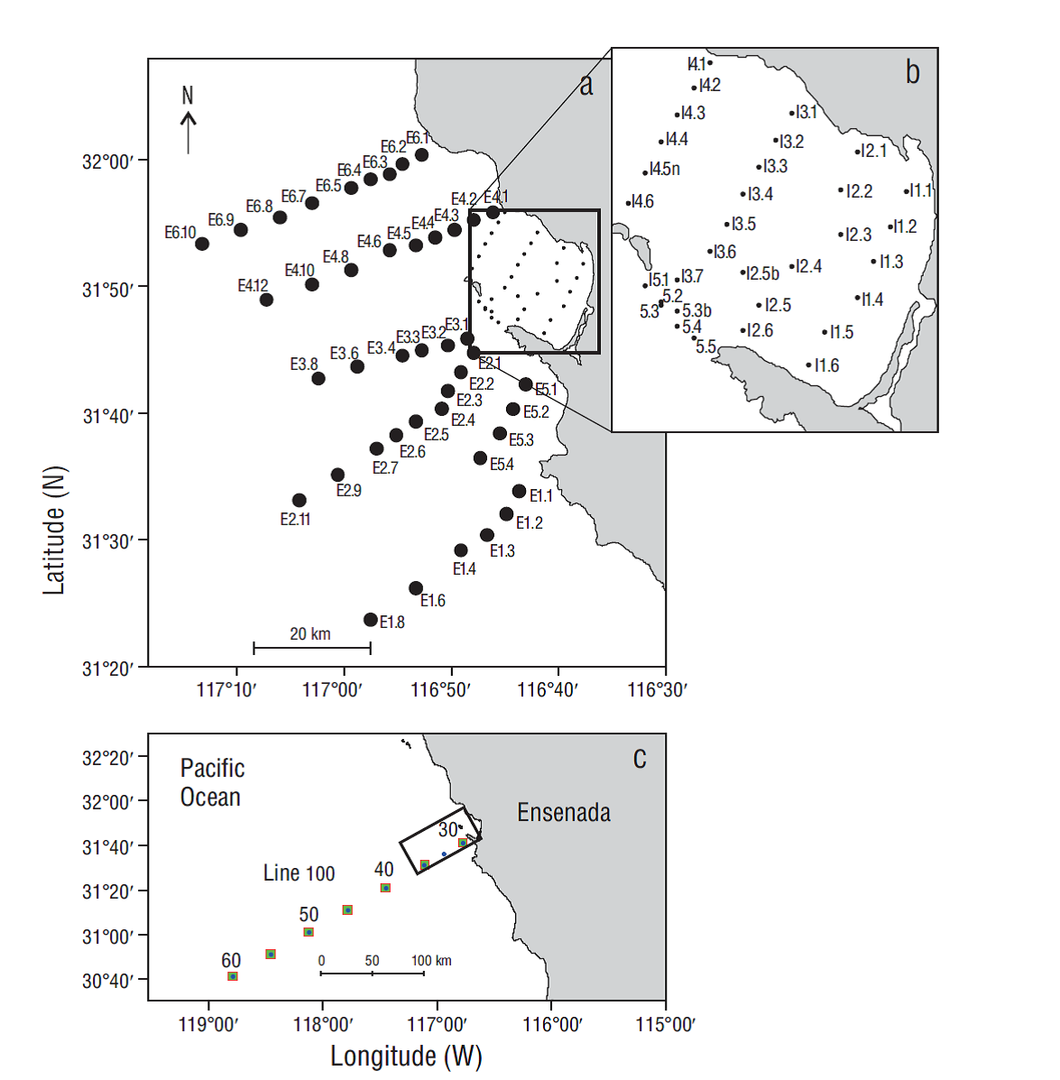
Figure 1 Map showing the IMECOCAL transects and the sampling stations in Todos Santos Bay where the CTD measurements were recorded in 2011: (a) outer stations, (b) inner stations. (c) Hydrographic stations along line 100 of the IMECOCAL program. The rectangle in (c) indicates the stations (100.30, 100.32, and 100.35) that were used as climatological references.
During periods of intense wind blowing parallel to the coast, wind promotes the flow of water from outside TSB to the innermost part of the bay (Flores-Vidal et al. 2015). When winds weaken, this water (of upwelling origin) can remain trapped in TSB. The characteristics of the CCS are thus restricted to the area adjacent to TSB and, as a result, the physical and biochemical properties of water can be different in and out of the bay. For example, in 2008, there were differences in average sea surface temperature in (17.74 ± 0.42 ºC) and out (14.67 ± 0.52 ºC) of TSB (Delgadillo- Hinojosa et al. 2015). The difference in temperatures was due to the heat the CCS water gained as it entered TSB. The possible influence of upwelled waters toward the inner part of TSB has also been reported (Zaytsev et al. 2003, Perez-Brunius et al. 2007).
Sampling design
During 2011, 4 cruises were carried out aboard the R/V Francisco de Ulloa to characterize the spatial and temporal distribution of the CO2 system variables in TSB. The cruises were classified based on the seasonal period in which they were carried out: February (winter), May (spring), August (summer), and November (autumn). During these cruises temperature (ºC), salinity, and dissolved oxygen (μmol·kg-1) were measured by making conductivity, temperature, and depth (CTD SBE 9/11) casts in TSB and the adjacent coastal zone (Fig. 1). Seventy-four hydrographic stations were sampled during each cruise, 32 of which were located in TSB (inner stations) and the rest were distributed into 4 transects perpendicular to the coastline and 1 transect at the southern entrance. During each campaign, water samples were collected with 5-L Niskin bottles at standard depths (0, 10, 20, 50, 100, 150, and 200 m) to determine DIC and total alkalinity.
Water masses
Water masses in the study area were identified with a hydrographic analysis using temperature and salinity diagrams (T-S diagrams) and the classification by Durazo and Baumgartner (2002).
Dissolved inorganic carbon and total alkalinity analyses
DIC in the water samples was analyzed using the coulometric system described by Johnson et al. (1987), while total alkalinity was measured by potentiometry according to Hernández-Ayón et al. (1999). Calibrations for both analyses were done with certified reference material (Marine Physical Laboratory at Scripps Institution of Oceanography, headed by Dr. Andrew Dickson), with which a ±3 μmol precision and a 1.5% error were obtained. Ωa was calculated using the CO2Sys program (Lewis and Wallace 1998) and by taking the DIC-total alkalinity pair, temperature, salinity, pressure, and the dissociation constants by Mehrbach et al. (1973) into account.
Empirical model for the reconstruction of pH, Ωa, and dissolved inorganic carbon
With the CTD hydrographic data pH, Ωa, and DIC were calculated for each of the 4 cruises using the empirical relationships proposed by Alin et al. (2012):
where T is temperature (ºC), S is salinity, O2 is dissolved oxygen (μmol·kg-1), σθ is the potential density anomaly (kg·m-3), and α is the coefficient estimated for each model; subscript r indicates reference values and superscript est indicates estimated values (Alin et al. 2012). The estimations provide information on the average state of the CO2 system variables in waters between 15 and 500 m depth for any moment between 1997 and 2017. The equations can be used for sites with limited observations on the carbon variables, and these variables in turn can subsequently be used to calibrate the model. Validation of this methodology was done by comparing the DIC and Ωa values from the samples collected during the oceanographic campaigns with the values produced by the model (Fig. 2). On Figure 2 we also superimposed the data obtained for line 100 during the National Oceanic and Atmospheric Administration (NOAA, USA) (WC200705) cruise in May-June 2007.
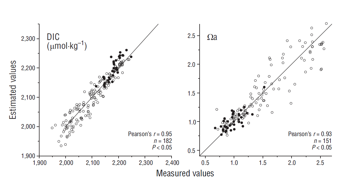
Figure 2 Measured versus estimated values for dissolved inorganic carbon (DIC) and aragonite saturation state (Ωa). White circles correspond to samples collected off the coast of Baja California during a cruise carried out by the North American Carbon Program in May 2007 and black circles correspond to samples collected during the present study in 2011.
The statistical analysis shows that the DIC and Ωa values obtained with the empirical relationships were similar to the measured values obtained during the 4 cruises (DIC: rpearson = 0.95, n = 182, P < 0.05; Ωa: rpearson = 0.93, n = 151, P < 0.05).
Oceanographic climatology off Todos Santos Bay
Line 100 of the IMECOCAL (Spanish acronym for Mexican Investigations of the California Current) program corresponds to the section nearest TSB, and hydrographic data for it covers from 1997 to 2016 (Fig. 1c). Therefore, in addition to average data, temperature and salinity measurements obtained in 2011 at the nearshore stations on this line (stations 100.30, 100.32, and 100.35) were used as reference for oceanographic conditions in our study region.
Our study in TSB was carried out under La Niña conditions. This was evidenced by Oceanic Niño Index (ONI) values ranging from -0.5 to -1.5 (Fig. 3), which indicate the presence of a negative sea surface temperature anomaly (http://www.cpc.ncep.noaa.gov/products/analysis_monitoring/ensostuff/ensoyears_1971-2000_climo.shtml ). In the analysis we also included the monthly upwelling index for the past 7 years (https://www.pfeg.noaa.gov/products/PFELData/upwell/monthly/upanoms.mon ), together with the ONI and upwelling index standardized anomalies for contrast with ONI (Fig. 3).
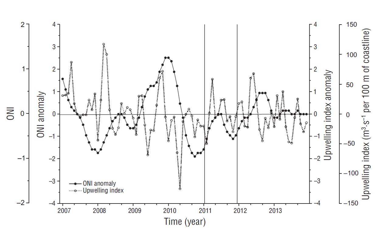
Figure 3 Monthly Oceanic Niño Index (ONI) anomalies (solid line) and upwelling index anomalies (dotted line) for the period from January 2007 to December 2013. Vertical lines indicate the sampling period for our study. Upwelling indices were obtained from https://www.pfeg.noaa.gov/products/PFELData/upwell/monthly/upanoms.mon and ONI were obtained from http://www.cpc.ncep.noaa.gov/products/analysis_monitoring/ensostuff/ensoyears_1971-2000_climo.shtml.
To assess if the physical changes that occurred in 2011 were influenced by La Niña conditions, the relationship between the depth of the Subarctic Water lower limit (ZSAW, defined by the 25.9 kg·m-3 isopycnal) and the ONI values for each cruise was estimated. This analysis was done for the winters (December and February) in the period from 1998 to 2012 at stations 100.30, 100.32, and 100.35 of the IMECOCAL program. The depth of the core of the California Countercurrent (ZCCc, defined by the 26.5 kg·m-3 isopycnal) was also located. Isopycnals were chosen by following the definition by Durazo (2015) and by detecting the temperature and salinity limits in the climatology of the water masses determined by the T-S diagrams.
Results
Hydrographic conditions (2011) and climatological conditions (1997-2016)
The T-S diagrams for transect E1 in the 4 cruises and for the IMECOCAL stations (100.30, 100.32, and 100.35) showed seasonal variation (Fig. 4) associated with the presence of less saline (~33.3) and colder (15 ºC) water. Anomalously cool and less saline Subarctic Water (SAW) was observed from the surface to 200 m depth in winter (Fig. 4a), from the surface to ~100 m depth in spring (Fig. 4b), and from ~100 m down to 200 m depth in summer (Fig. 4c). In autumn, the depth of the 25.0 kg·m-3 isopycnal was similar to that of the climatological record. By contrast, the T-S diagram for transect E1, located to the south of TSB, showed hydrographic conditions that were close to the climatological average (Fig. 4b, d, f, g).
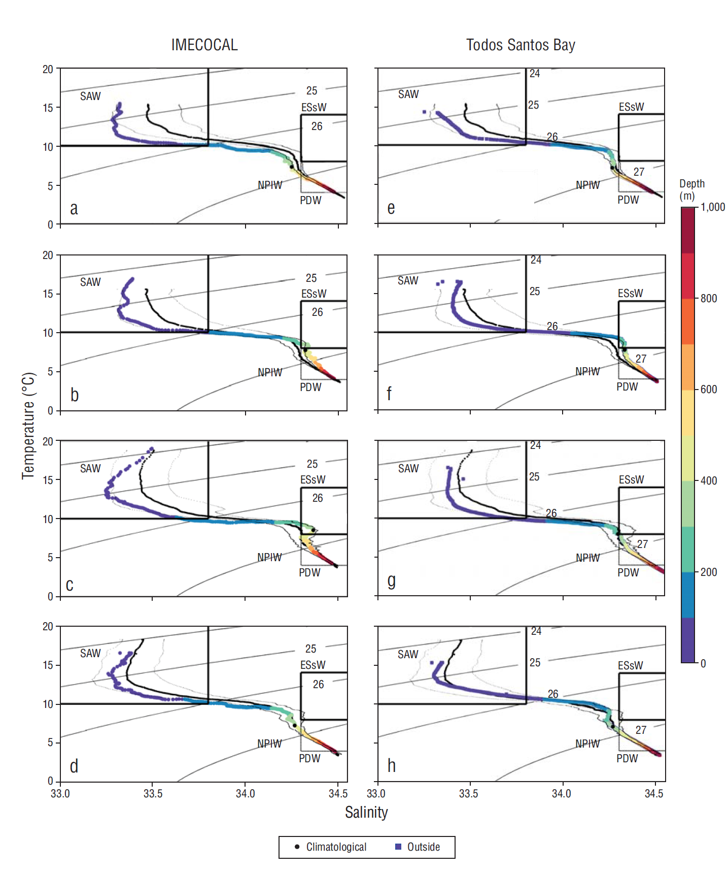
Figure 4 Temperature-salinity curves with reference to depth measured along line 100 of the IMECOCAL program during 2011 (a, b, c, d) and along transect E1 outside Todos Santos Bay in 2011 during winter, spring, summer, and autumn (e, f, g, h). The black continuous line represents the long-term mean obtained from data recorded by the IMECOCAL program between 1998 and 2017 and the thick black discontinuous lines represent the standard deviation. Water masses are Subarctic Water (SAW), Equatorial Subsurface Water (ESsW), North Pacific Intermediate Water (NPIW), and Pacific Deep Water (PDW).
Seasonality of water masses
The SAW lower limit was located at different depths in every season (Fig. 5). For example, in winter, on transect E1, there was an upward movement of ZSAW from 100 m to ~50 m toward the coast, whereas ZCCc sank from 200 to 250 m toward the coast. The upward movement of isopycnals was less pronounced in spring than in winter; ZSAW rose from 100 to ~60 m, but ZCCc remained somewhere between 170 and 200 m (Fig. 5). In summer, ZSAW persisted at ~70 ± 7 m and ZCCc was detected near the coast at ~300 m. In autumn, ZSAW (~125 m) was deeper and ZCCc (~250 m) was slightly shallower than in the previous season.
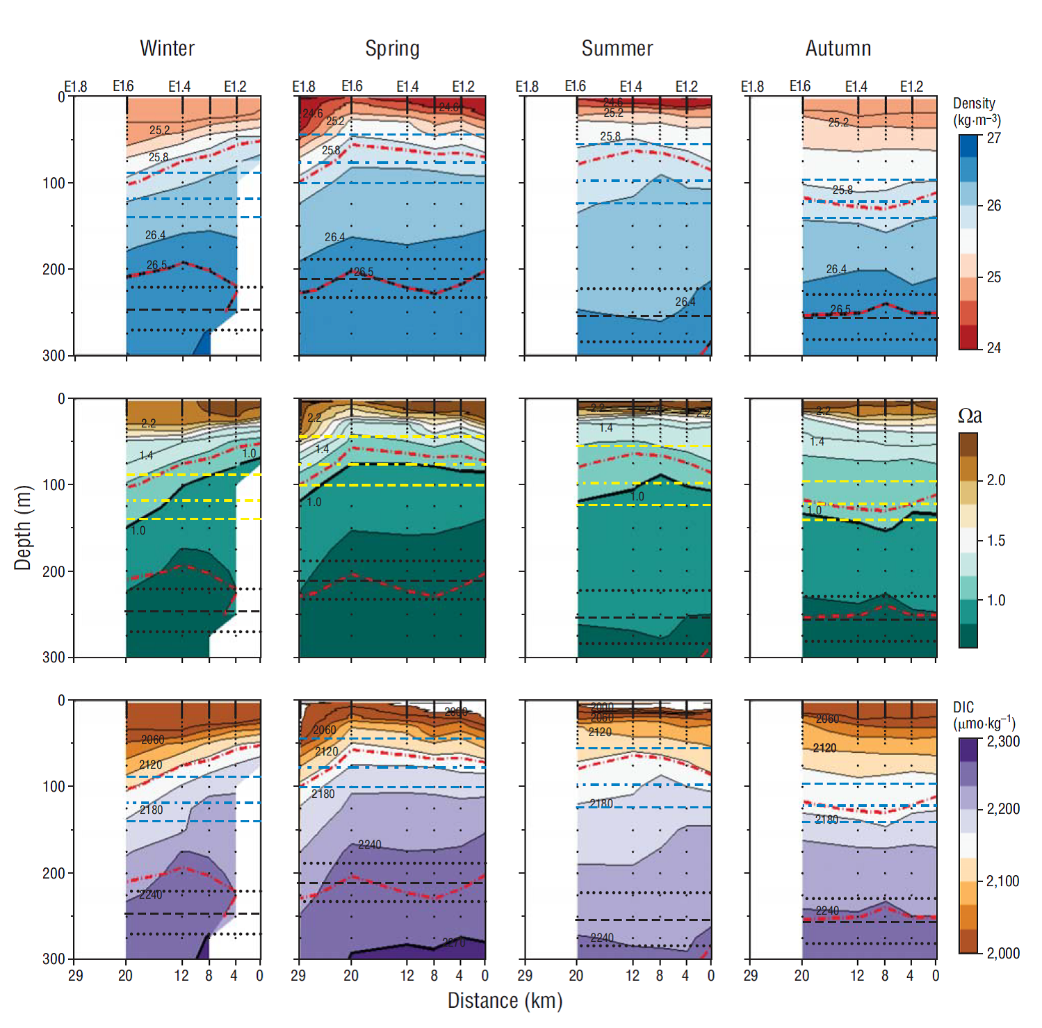
Figure 5 Seasonal variations of density, aragonite saturation state (Ωa), and dissolved inorganic carbon (DIC) by depth along transect E1 (southern portion of our study area) in Todos Santos Bay. The red dash-dot lines indicate the 25.9 kg·m-3 and 26.5 kg·m-3 isopycnals, which correspond to the lower limit of the Subarctic Water and to the locations of core of the California Countercurrent, respectively. The horizontal dashed lines represent the average depth of these isopycnals during the 1997-2011 period at stations 100.30-100.35 of the IMECOCAL program.
Seasonality of the CO2 system variables
The seasonal variation of the CO2 system variables was consistent with the distribution of the water masses. For example, water with high DIC content (~2,180 µmol·kg-1) and low Ωa values was detected in winter, when Isopycnals rose to ~80 m depth toward the coast (Fig. 5). The shallowest ZΩa value near the coast was not found during the season with the most intense coastal upwelling (spring-summer), but in winter. Furthermore, the greatest upward movement of isopycnals toward the coast coincided with the season during which La Niña was most intense.
Influence of interannual conditions
The relationship between ZSAW and ONI showed that when ONI values were negative ZSAW shoaled (Fig. 6). For example, during the 2010-2011 winter and under La Niña conditions, ZSAW was located at 102 m and ONI values were -1.3 ºC. Conversely, in the winter of 1998, under El Niño conditions, ZSAW was located at 162 m and ONI was +2.1 ºC. According to the linear regression analysis, ONI explained 60% (r2 = 0.6, P < 0.01, n = 12) of the seasonal variability in the position of ZSAW.
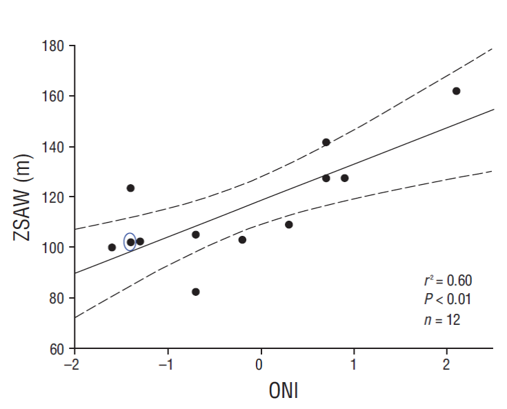
Figure 6 Average depth of the Subarctic Water boundary corresponding to the 25.9 kg·m-3 isopycnal (ZSAW) plotted against the Oceanic Niño Index (ONI). Data are for the cruises carried out by the IMECOCAL program along line 100 from December to February 1998-2012. The blue circle denotes the values for 2011.
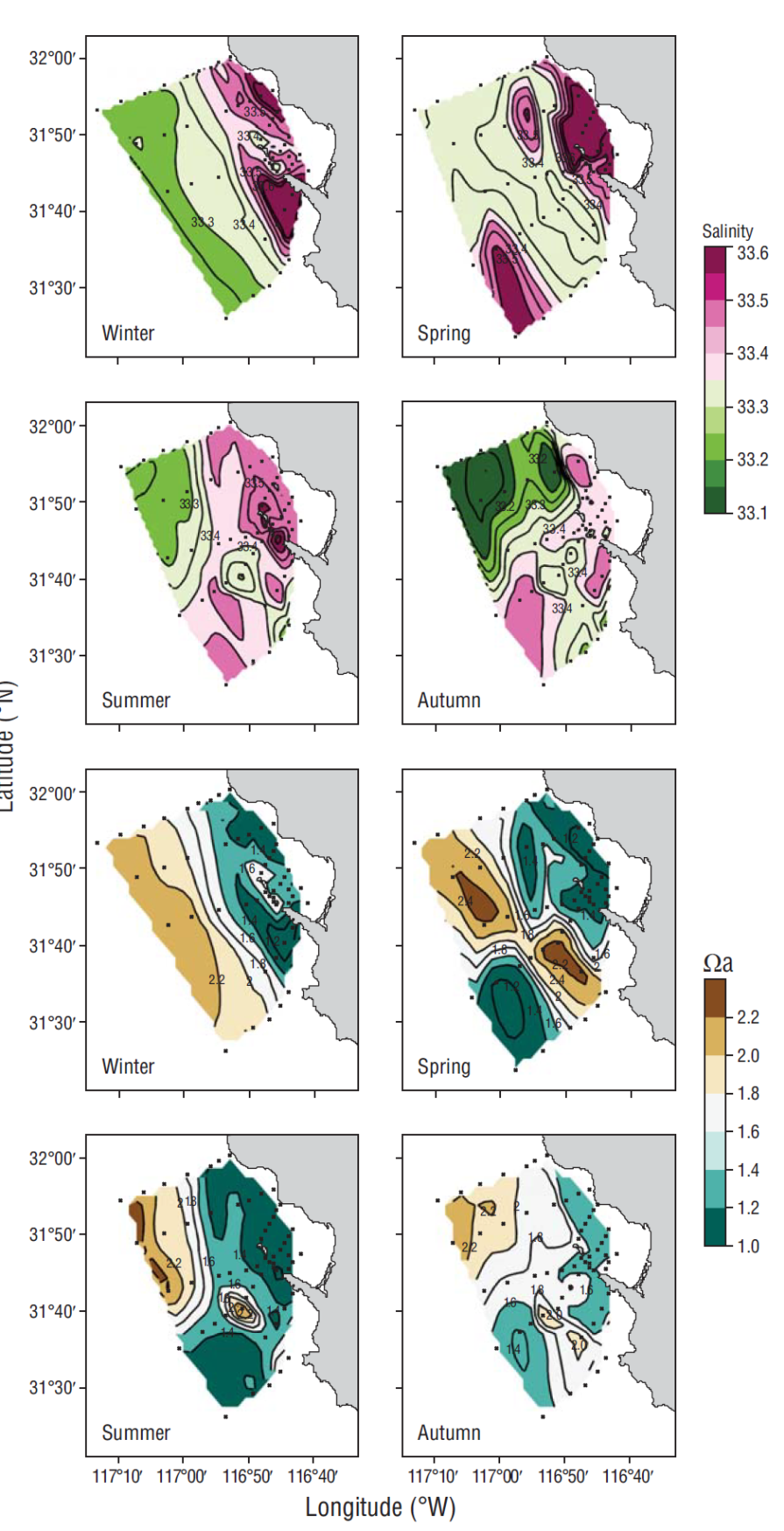
The inner sampling stations and those adjacent to TSB had saline waters (>33.4) and Ωa values less than 1.6. However, the opposite scenario was observed outside TSB because of the dominance of SAW (mainly in winter) (Fig. 7). During winter, a north-south front parallel to the coast separated TSB water from adjacent waters, which were low in salinity (<33.3) and high in Ωa values (>2.2). Furthermore, characteristics similar to the winter conditions were found in spring. In summer, less-saline water (~33.3) with Ωa values of ~2.2 was distributed mainly to the northwest of the sampling zone. The opposite of what was observed during summer occurred during autumn, with less-saline water in the study area occurring from north to south as an intrusion (Fig. 7d).
Vertical variation of ZΩa
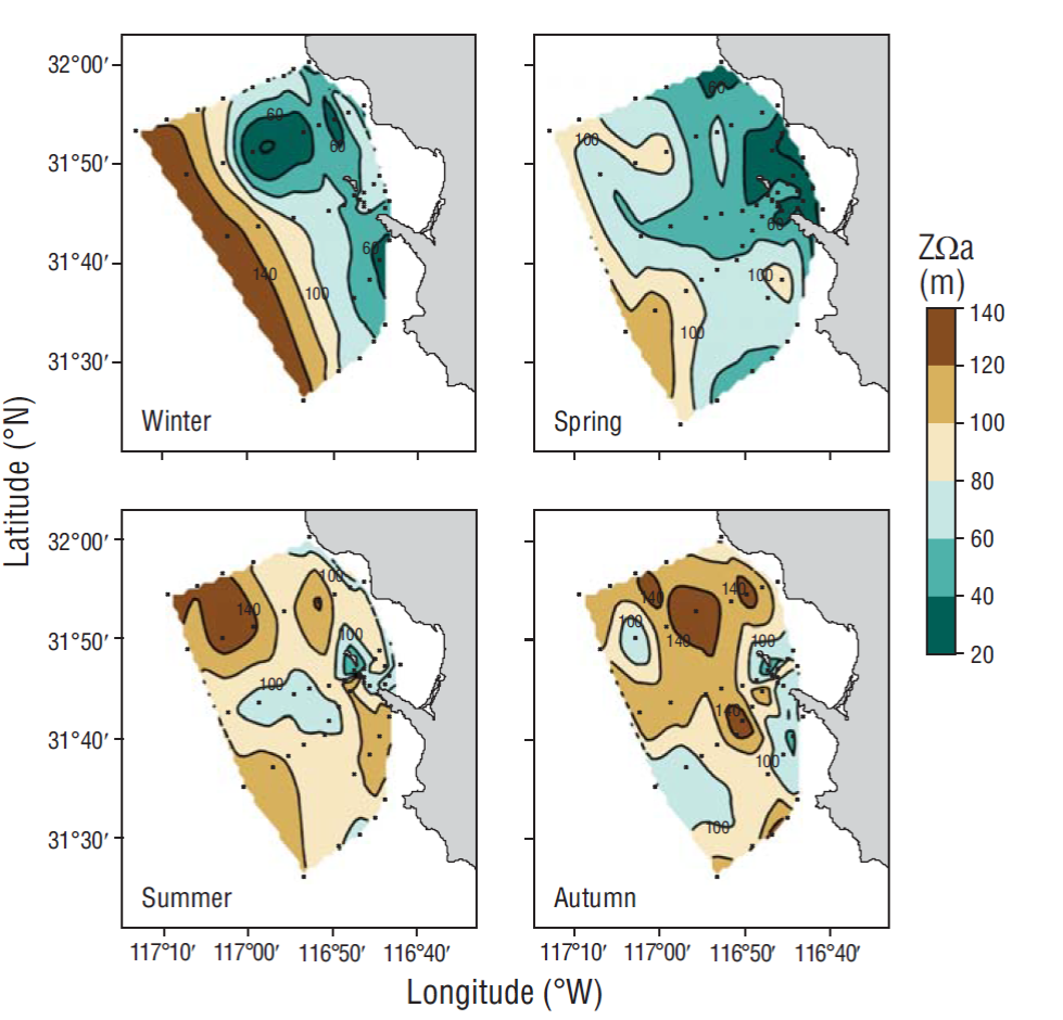
ZΩa fluctuated spatially and seasonally (Fig. 8). In winter it was less than 60 m close to shore and it gradually increased offshore until reaching values >140 m. This scenario changed in spring, with a shallower horizon throughout most of the study area. In TSB ZΩa was shallower (30 m) but in the more oceanic region it was ~80 m. In summer, ZΩa was generally deeper in the northwestern area (>140 m), and it showed a positive gradient toward the south (120-100 m). However, the gradient was less pronounced toward the Todos Santos Islands, where it was located at shallower depths, between 60 and 80 m. In autumn, ZΩa was located at >140 m in the northeastern and central portions of the sampling area where the outer stations were located. ZΩa was shallower toward TSB.
Contrast between the oceanography in and out of Todos Santos Bay
The inner and outer TSB stations showed differences in physical and chemical variables only during winter and spring (Fig. 8). The most relevant observation was that, in winter and spring, temperature and Ωa were lower and salinity was higher in TSB than in the oceanic waters outside the bay (Fig. 8). Salinity helped understand the differences we found. For example, the highest salinity variability (33.0-34.5) was found at stations outside TSB; however, toward the bay most salinity values were higher than the average, and Ωa (0.5-3.0) and temperature (3-19 ºC) values were higher with respect to the climatological values by 0.5 units and 4 ºC, respectively.
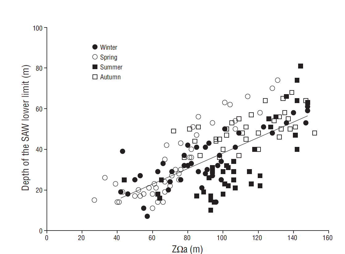
Relationship between ZSAW and ZΩa
The 2011 La Niña conditions were more intense in winter; this was reflected in the position of ZSAW, which was shallower compared to the climatology for that season (Fig. 9). This difference was detected by comparing ZSAW with ZΩa. ZSAW and ZΩa were located at approximately the same position during the winter (rpearson = 0.78, n = 42, P < 0.05), spring (rpearson = 0.70, n = 52, P < 0.05), and summer (rpearson = 0.78, n = 49, P < 0.05) cruises; this was not the case for autumn (rpearson = 0.54 n = 46, P < 0.05) (Fig. 9).
Discussion
Influence of Subarctic Water on the position of ZΩa
In this study we found that the distribution of ZΩa corresponded with the distribution of the characteristics of the water masses in the region. Therefore, higher proportions of SAW in the water column result in deeper positions of ZΩa. This behavior was observed mainly in winter and spring 2011, when the California Current was anomalously more intense during La Niña, as was reported in other studies for the southern part of the California Current (Bjorkstedt et al. 2012, Jacox et al. 2016, Rudnick et al. 2017). During La Niña conditions, SAW predominated in the more oceanic section, but water in TSB was saltier. These conditions consequently changed the chemistry of carbonates.
Oceanographic conditions in 2011
In winter and spring, SAW predominates off the northern coasts of Baja California, while in autumn and winter the California Countercurrent is more intense and transports Equatorial Subsurface Water (ESsW) in a northward direction (Linacre et al. 2010a, Durazo 2015). However, under the 2011 La Niña conditions, the oceanographic scenario was different. Strong anticyclonic wind anomalies were present in the North Pacific, prompting cooling conditions, as reflected by the negative sea surface temperature anomalies in the CCS that lasted until September-October 2011 (Bjorkstedt et al. 2012).
The negative ONI anomalies (-1.5 ºC) recorded during 2011 were slightly weaker than those detected during the 2008 La Niña event (ONI values of approximately -2 ºC). During this 2008 event, there were pulses of DIC-rich water, with high nutrient concentrations and noticeable effects on the diversity of the phytoplankton community (Linacre et al. 2010a , b; 2012). The results of this study suggest that the most evident effect of the 2011 La Niña event was the presence of water that was colder and less saline than normal, particularly in winter. These results are consistent with the fact that the 2011 La Niña event was more intense in winter and gradually lost intensity toward the end of that year.
In the present study the thermohaline structure above 300 m depth was formed by 2 water masses, SAW, which is less saline (~33.3), and ESsW, which shows higher salinity values (~34.4), in agreement with what other authors have reported (Durazo and Baumgartner 2002, Durazo 2015). Both of these water masses are transported by the California Current and the California Countercurrent, respectively, along the coasts of Baja California (Durazo and Baumgartner 2002, Pérez-Brunius et al. 2006, Durazo 2015). Several studies have indicated that, over the continental shelf of Baja California, from spring to autumn, the poleward subsurface countercurrent is more intense and advects ESsW (Lynn and Simpson 1987, Linacre et al. 2010a, Durazo 2015). At depths of ~150 m, ESsW mixes with SAW and forms transitional water, which we consider is responsible for values of Ωa = 1. The proportion of this water masses will determine if ZΩa deepens when SAW predominates or if it shoals when the ESsW signal intensifies. However, the proportion and distribution of water masses on the coasts of Baja California change during events like El Niño and La Niña (Durazo and Baumgartner 2002). Therefore, a combination of interannual conditions promotes changes in the magnitude of the carbonate system variables in the water column of the southern portion of the CCS.
An example of the influence of interannual conditions in the southern portion of the CCS in relation to the signal of the CO2 system was reported by Friederich et al. (2002) for the coasts of Monterey Bay (California, USA). These authors carried out CO2 partial pressure (pCO2) surface measurements during the 1997-1998 El Niño and La Niña events and reported high surface pCO2 concentrations during La Niña conditions and values near equilibrium with respect to the atmosphere during El Niño conditions because there were no upwelling events during that period. Another example is shown in a study carried out on the coasts of San Diego (California, USA) during the 2010 La Niña conditions, in which Nam et al. (2011) detected low pH values and the upward movement of isopycnals toward the coast. Similarly, another study carried out during the 2011 La Niña event on the coasts of San Diego detected temperature and salinity anomalies of -1.5 and -0.1, respectively (Rudnick et al. 2017), and the upward movement of the 26.0 kg·m-3 isopycnal by about 20 m from an average depth of 150 m (Jacox et al. 2016).
Interannual events undoubtedly affect the regional oceanography and, in turn, thermohaline variables and water chemistry. A recently published study on pCO2 measurements obtained during 2011 at the Ensenada station (Coronado-Álvarez et al. 2017) reported the presence of upwelling episodes with high CO2 fluxes (up to 3.8 mmol C·m-2·h-1) and low temperatures (~10 ºC). High pCO2 values indicate that pH was lower during that year, as were Ωa values.
Our study on TSB during the 2011 La Niña event suggests the presence of anomalously cold, less-saline SAW in the most oceanic region and saltier water in TSB. Also in TSB, pH (<7.7) values were the lowest and high DIC concentrations (2,200 µmol·kg-1) were detected at shallower depths near the coast (≤100 m) in winter and spring.
Comparison of physical and chemical conditions in and out of Todos Santos Bay
La Niña effects were reflected on the hydrographic conditions at both the IMECOCAL stations (coast and ocean) and the stations adjacent to TSB. Using the T-S diagrams, we detected that the characteristics of water masses at the IMECOCAL stations were similar to those detected at stations outside TSB. However, during winter and spring, water was more saline in TSB and near the coast (Fig. 8). As mentioned above, this could be attributed to the entrance of subsurface water to TSB during upwelling events, which contributed to the perpetuity of this water in TSB due to water recirculation in the bay (Delgadillo-Hinojosa et al. 2015).
The results of this study suggest that ZΩa was located at 30 m, that is, 10 m shallower than what Feely et al. (2008) reported for waters off TSB and adjacent areas. There were no previous records of ZΩa for TSB, nor that it could be so shallow (30 m), as reported in this study. This could pose a threat to organisms in the area that use carbonate to calcify their structures in their first life stages. For example, larval development for the oyster Crassostrea gigas requires optimum values of Ωa > 1.6 (Barton et al. 2012). Therefore, if values of Ωa = 1 at ~20 m depth during intense upwelling events in TSB, conditions may be unfavorable for some calcifying species that inhabit this area.
This study contributes to the advancement of knowledge on the carbonate system in TSB. Though the results of this study are based on punctual observations and model reconstructions, information here shows that characteristics during events such as La Niña can produce different oceanographic scenarios that affect the carbonate system in TSB coastal waters. In addition, the results suggest that ZΩa was particularly shallow during the 2011 La Niña event, mainly at the beginning of the year (winter), and this could potentially influence the proper development of the larval stages of calcifying organisms in the area.

