Artículos

 

Deriving sediment quality guidelines in the Guadalquivir estuary associated with the Aznalcóllar mining spill: A comparison of different approaches

 

Obtención de guías de calidad de sedimento en el estuario del Guadalquivir asociadas con el vertido minero de Aznalcóllar: Una comparación de diferentes métodos

 

I. Riba^1*, V. Zitko², J.M. Forja¹ and T.A. DelValls¹

 

¹ Departamento de Química Física, Facultad de Ciencias del Mar, Universidad de Cádiz, Apartado 40 11510 Puerto Real, Cádiz, España. *E-mail: inmaculada.riba@uca.es

² ChemEnv, 114 Reed Ave, St. Andrews, N.B., E5B 1A1, Canada.

 

Recibido en febrero de 2003;
aceptado en abril de 2003.

 

Abstract

Concentrations of heavy metals (Fe, Zn, Cd, Pb, Cu and Mn) and sediment toxicity tests (mortality of amphipods, Ampelisca brevicornis, of clams, Scrobicularia plana, and of fish, Solea senegalensis) were used to derive sediment quality guidelines (SQGs). The approaches are based on the determination of LC50, on the application of a multivariate analysis (MAA), and on the Threshold Effect Level Quotients (TELQs). All approaches lead to consistent SQGs. The range of concentrations established with MAA results in narrower uncertainty ranges. Sediment toxicity estimated by TELQs is in good agreement with that determined experimentally. In terms of the toxic mud concentration, the maximum and minimum LC50s (for fish EC50s) are 1.07% and 0.44% for amphipods, 5.75% and 1.25% for clams, and 7.24% and 1.97% for fish, based on dry weight. However, heavy metal concentrations or ranges should be used only as a first tier in a "weight-of-evidence" approach to determine the environmental quality in aquatic systems. The use of SQGs for the management of these systems should be taken with care, especially those used for the management of dredging processes.

Key words: sediment quality guidelines, sediment contamination, sediment toxicity, multivariate analysis, LC50.

 

Resumen

Se han utilizado las concentraciones de los metales pesados: Fe, Zn, Cd, Pb, Cu, Mn, y los resultados de toxicidad (mortalidad de anfípodos: Ampelisca brevicornis, coquinas: Scrobicularia plana, y peces: Solea senegalensis) para obtener guías de calidad de sedimento (SQGs). Los métodos utilizados se basan en la determinación de LC50s, en la aplicación del análisis multivariante (MAA), y en la utilización de los coeficientes del nivel del umbral de efecto (TELQs). Todos los métodos permiten obtener las guías de calidad. De los resultados obtenidos en la aplicación del MAA se obtienen áreas de incertidumbre con intervalos más estrechos. La toxicidad de sedimento, estimada por el método TELQs, presenta una buena correlación con aquella determinada experimentalmente. En los términos de concentración de lodo tóxico, los valores máximos y mínimos de LC50s (para peces EC50s) son 1.07% y 0.44%, para anfípodos; 5.75% y 1.25%, para coquinas; y 7.24% y 1.97% para peces, y éstos vienen expresados como porcentaje de lodo tóxico en peso seco. Sin embargo, estos intervalos de concentraciones mencionados debieran ser utilizados en un primer paso cómo un método basado en "el peso de la evidencia" cuando se utilizaran para establecer la calidad ambiental en sistemas acuáticos. Cuando el propósito sea la utilización de estas guías de calidad de sedimento en la gestión de dragados, éstas deben utilizarse con precaución.

Palabras clave: guías de calidad de sedimento, contaminación de sedimento, toxicidad de sedimento, análisis multivariante, LC50.

 

Introduction

During the last decades there has been some debate about the use of the words criteria, guidelines, site-specific values, etc., as a final proposal in sediment quality studies regarding the protection of the environmental quality in aquatic ecosystems (Chapman, 1991). The term sediment quality guidelines (SQGs) is now widely accepted. It gives the range of concentrations of chemicals associated with the presence or absence of adverse biological effects (Wenning and Ingersoll, 2002). Recent reports suggest that SQGs continue to be widely used, since they give reasonable predictions of the potential damage associated with chemicals in sediments (Fairey et al., 2001). However, it is still necessary to establish the appropriate use and limitations of SQGs as a management tool. The site specificity of SQGs should be re-assessed and discussed, particularly for special areas such as estuaries, highly influenced by large gradients of natural variability (salinity, pH, etc.) Such variability can affect the fate and effect of the sediment contaminants.

LC50s (or EC50s for sublethal effects, but for the sake of brevity only the term LC50 is used) are widely used to assess the adverse biological effects or hazards of contaminants. LC50s are based on sets of toxicological data and are, together with data on exposure, used to predict potential risks of contaminants. In a risk assessment, LC50s (a measure of hazard) are usually combined with contaminant concentrations (a measure of exposure) into toxic units or quotients (TUs, for sublethal effects the term Effect Levels may be used). TUs are ratios of concentrations of chemicals to their respective LC50s; they have been widely used for the management of risk and regulatory decisions. For instance, oil dispersant may be approved for use only on the basis of its LC50s for different organisms. On the other hand, multivariate analysis approaches (MAA), as well as "consensus", have been used to develop SQGs, which establish concentrations or ranges of concentrations of chemicals associated with adverse effects. The latter are usually defined as the Threshold Effect Level (TEL), Effects Range Low, Probable Effects Level, Effects Range Median, and Apparent Effects Threshold (Long et al., 1995; DelValls and Chapman, 1998; NOAA/HAZMAT, 1999; Ingersoll et al., 2001). As in the case of LC50s, the MAA-derived range of concentrations of contaminants associated with adverse biological effects can be used to establish the associated risk (DelValls et al., 1998; Riba et al., 2002a). The mean of TUs is used to assess the risk of complex chemical mixtures (Fairey et al., 2001).

During the monitoring of the Aznalcóllar mining spill (April 1998), an integrated assessment was conducted in the Guadalquivir estuary to determine the impact of the heavy metals related to the accidental spill. During this study, sediment samples from the estuary and different concentrations of the spilled toxic mud diluted in a clean sediment were analyzed and their toxicity was determined. The aim of this work was to establish the feasibility of using these data to predict sediment quality in the area. The error associated with the different approaches employed to derive SQGs was estimated and the role of SQGs in the management of the risk of heavy metals from the spill was evaluated.

 

Material and methods

Approach

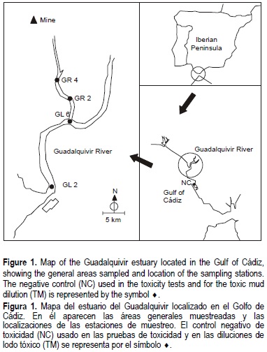
The present study was performed at four stations (GL2, GL6, GR2 and GR4) in the Guadalquivir estuary, SW Spain (fig. 1). Toxic mud was collected from an impacted area, located 40 km away from the Aznalcóllar mine tailing pond. The mud was diluted by a clean sediment from the Bay of Cádiz (fig. 1) to yield concentrations of 0.3%, 1.8%, 7.9%, 20% and 32% dry weight. The dilutions were performed in the containers for the toxicity tests. The mixtures were homogenized in water to be used in the tests. A detailed description of the dilution procedures, the collection of the samples, the chemical analysis and the toxicity tests are reported by Riba et al. (2002b). A summarized description of these processes and techniques is shown in table 1.

LC50 approach

The LC50 value is the concentration of toxic mud that results in the mortality of 50% of the animals tested. The LC50s are calculated by linear regressions of the logarithms of the concentration of toxic mud on declining probit values, by the EPA-Probit analysis program (version 1.5, Ecological Monitoring System Laboratory, EPA, Cincinati, Ohio). This software determines the value of LC50 and the maximum and minimum values of the 95% confidence interval. We have used these maximum and minimum values to derive the SQGs. The concentration of toxic mud corresponding to the maximum LC50 was used to calculate the concentration of the heavy metals associated with the toxic effect, and was defined as "major adverse biological effects". Similarly, the minimum value of LC50 yielded the concentration of heavy metals not associated with the toxic effect and was defined as "no or minimal adverse biological effects". The difference between both is the uncertainty interval.

To derive SQGs for a metal at a given LC50 (SQG(M)_LC50), the following expression was used:

where C_TM is the concentration of the metal in the toxic mud and C_c is the concentration of the metal in the control sediment used to dilute the toxic mud. These concentrations were previously reported by Riba et al. (2002b); CTM and CC are, respectively, 21618 and 41.6 mg kg^-1 for Zn, 45.7 and 0.1mg kg^-1 for Cd, 2033 and 9.5 mg kg^-1 for Cu, and 7873 and 71.9 mg kg^-1 for Pb, dry weight. The %TM and %C correspond to the percentage of toxic mud and control, respectively, for a given value of LC50. The values of LC50 are obtained for each bioassay and expressed as percentage of toxic mud. As an example we show the derivation of SQGs for Zn from the LC50 calculated for clams (maximum 5.75% and minimum 1.25%). The maximum is related to a percentage of toxic mud of 5.75%, so the percentage of control sediment is 94.25%. The concentration of Zn in the toxic mud is (see above) 21618 mg kg^-1 and the concentration of Zn in the control sediment is 41.6 mg kg^-1. From the above equation, the SQG values are 1282 and 311 mg kg^-1 for the maximum and minimum LC50, respectively. The uncertainty interval is the difference between these two values. The same calculations were carried out for the other metals.

Multivariate analysis approach

Assumptions in the application of the MAA to the data are that the heavy metals measured are those responsible for the effects observed and outweigh the influence of natural physicochemical factors. Other co-varying and not quantified chemicals may have had an influence on the effects observed. The effects of potential interactions of the mixture of metals (synergism, additivity, antagonism) are unknown and the MAA assumes that they act independently. Such considerations were previously reported in the performance of multivariate analysis to link chemical and toxicological data (Zitko, 1994).

The chemical and toxicological data were analyzed by statistical analysis (principal component analysis, PCA) to explore the patterns of the variables (heavy metals: n = 6; biological effects: n = 3). The objective of PCA is to derive a reduced number of new variables as linear combinations of the original variables. This provides a description of the structure of the data with the minimum loss of information. The PCA was performed on the correlation matrix; i.e., the variables were centered (mean = 0) and scaled (standard deviation = 1) to be treated with equal importance. All analyses were performed using the PCA option of the FACTOR procedure, followed by the basic setup for factor analysis procedure (P4M) from the BMDP statistical software package (Frane et al. , 1985). The samples included the five toxic mud concentrations (0.3%, 1.8%, 7.9%, 20% and 32%) and the four sediment samples collected in the Guadalquivir estuary (GL2, GL6, GR2 and GR4). The resulting sorted, rotated factor loadings are coefficients correlating the original variables and the principal factors in this analysis. The variables are reordered so the rotated factor loadings for each factor are clustered together. In the present study, we selected to interpret a variable or group of variables as those associated with a particular factor where loadings were ≥ 0.3, corresponding to an associated explained variance over 65%. This approximates Comrey's (1973) cut-off of 0.55 for a good association between an original variable and a factor, and also takes into account discontinuities in the magnitudes of loadings approximating the original variables.

To derive the SQGs for the Guadalquivir estuary, a representation of the factor scores for each sample to the centroid of all cases for the original data is needed. We use the factor scores (prevalence) of principal factors to make three definitions: when the factor 3 (F3) scores are ≤ 0, the maximum concentrations of metals at those stations represent the maximum concentrations not associated with adverse effects. These are considered the concentrations below which biological effects are low or minimal and are described here as "no or minimal adverse biological effects". The minimal concentrations of metals at stations where the F3 scores are > 0 are considered concentrations causing "major adverse biological effects". The difference between the latter and the former is the interval of uncertainty.

Threshold Effect Level Quotient approach

In the third approach, a hypothetical concentration of the toxic mud in the samples from the estuary was calculated from:

where GLR is the matrix of the concentrations of the metals in the GLR samples, with dimensions [rows = metals = 4, columns = GL2, GL6, GR2, GR4 = 4]. The matrix TM [rows = 4, columns = 2] contains the composition of the toxic mud in the first column and that of the clean sediment in the second column. The matrix M [rows = fractions = 2, columns = GL2, GL6, GR2, GR4 = 4], which contains the proportions of the toxic mud and the sediment, is calculated by least squares.

A cubic spline interpolation was used to construct the toxicity curves encompassing the three lowest concentrations of the toxic mud.

 

Results and discussion

The results of the chemical and toxicological data used to derive SQGs for the Guadalquivir estuary are summarized in table 2. The percentages of mortality of amphipods and clams were used to calculate the LC50 for each organism. The lesion index percentage of damaged tissues (gills, intestine and gut) in the bottom-fish Solea senegalensis was used in a similar way to calculate the LC50. This is a sublethal effect concentration (EC50) that causes damage in all the tissues studied, in 50% of the fish.

The "no effect" and "major effect" concentrations as well as the uncertainty interval are given in table 3. It can be observed that the amphipods are the species most sensitive to the toxic mud. The sensitivity of clams and of fish in terms of sublethal effects, is lower. The widths of the uncertainty intervals are large for all three species. These results show that the LC50 approach can be used to derive SQGs associated with the mining spill. However, the wide uncertainty intervals between the concentrations associated with biological effects and those with no apparent effect produce large "gray intervals" for the determination of risk in impacted areas.

The application of PCA to the chemical and toxicological data represents the original variables (metals and toxicity tests) by three new variables, or principal factors (table 4). These factors explain 99.14% of the variance in the original data set. Negative values of sorted rotated factor loadings (negative salience) are as important as positive values (positive salience); however, in this analysis, the positive loadings are in general of larger magnitude than the negative loadings. The loadings following varimax rotation for the three factors are given in table 4. Each factor is described according to the dominant group of variables. The first principal factor, #1, is predominant and accounts for 88.32% of the variance. This factor combines the chemical concentrations of all the metals (Zn, Cd, Pb, Cu and Fe), except Mn, with all the biological effects (amphipods, Morty A; clams, Morty C; and fish lesions, LIT); it represents biological effects associated with chemicals from the accidental spill. The second factor, #2, accounts for 11.01% of the variance and combines only with the concentration of Mn but as negative loading. It represents a natural sedimentary matrix at the study site defined by variations in the Mn concentration and not associated with the biological effect measured in this study. The third factor, #3, accounts for 5.81% of the variance, and is a combination of four metals (Zn, Cd, Pb and Cu) and the three biological effects. The highest loading is associated with the mortality of amphipods, the rest of the loadings being lower than those grouped in factor 1. This factor was defined as the acute effect of the mining spill on the Guadalquivir estuary.

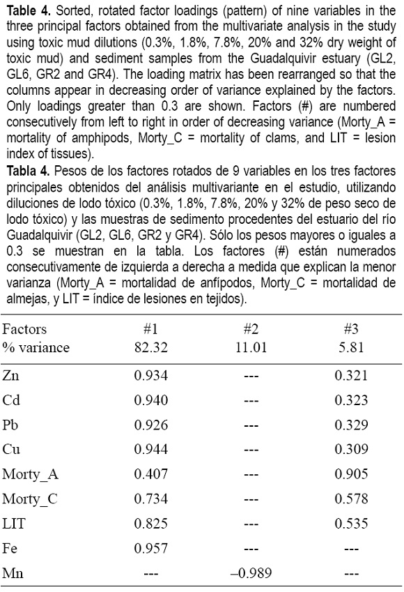
In order to confirm these factor descriptions and to establish the site-specific values of sediment quality, here defined as SQGs, in the Guadalquivir estuary, we propose a representation of estimated factor scores from each case (stations and dilutions of toxic mud) to the centroid of all cases for the original data (fig. 2). In general, values of factor #1 increase with increasing concentration of toxic mud, showing positive values at dilutions higher than 7.8% and a maximum value at the highest toxic mud dilution (32%). This factor score was always negative in all the sediment sampled in the Guadalquivir estuary. The other factor, which includes metal concentrations and biological effects in its definition, is factor #3. The value of this factor is positive at concentrations of toxic mud ≥ 1.8% and at station GR2, located in the Guadalquivir estuary. This confirms that factor #1 is associated with the toxic effects caused by metals in the toxic mud and that factor #3 is associated with the acute impact from the spill that affected the estuary.

To derive the SQGs, the factor scores were used and are shown in figure 2. When the scores of factor #3 (the factor showing relationships between the metals and adverse effects) are ≤ 0, the maximum concentrations of the metals at these stations are the maximum chemical concentrations not associated with adverse effects: "no or minimal adverse biological effects; not polluted". In contrast, to establish the minimal concentrations above which biological effects are always high, the minimum concentrations of the metals, at the stations where the score of factor #3 > 0, were selected and described here as "major adverse biological effects; highly polluted". The minimal and major effect concentrations, as well as the intermediate ranges of concentrations representing a "moderately polluted" interval of uncertainty, are shown in table 5.

To facilitate the understanding of the above-mentioned process to derive SQGs, we have described the calculation method for the case of Cd (table 5). The metal is included in factors #1 and #3 and therefore correlated to biological effect (table 4). Also, factor #3 is positive at concentrations of toxic mud ≥ 1.8 and at station GR2 (fig. 2), located in the Guadalquivir estuary. Its value is negative at dilution 0.3% and at the rest of the stations (GL2, GL6 and GR4) located in the estuary. The maximum concentration of Cd among these four cases is 0.8mgkg^-1 at station GR4 (table 2). This is the "no or minimal adverse biological effects" concentration (table 5). Similarly, to develop the "highly polluted" guideline, we find the minimum concentration of the metals (table 2) among the stations with factor #3 positive: 1.8%, 7.8%, 20%, 32% and GR2 (fig. 2), which for Cd is 0.9 mg kg^-1 at the toxic mud concentration of 1.8%. The "moderately polluted" uncertainty interval is the difference between these two concentrations. The SQG values for the other metals were derived in the same way (table 5).

To compare the prediction of risk associated with the heavy metals and expressed as SQGs by both approaches (LC50 and MAA), the "not polluted" and "highly polluted" guidelines, derived by the MAA, were compared to those calculated using the minimum and maximum values of LC50. The effectiveness was established comparing the uncertainty intervals determined by both approaches. An error quotient (ε) was defined as the uncertainty interval derived in the LC50 approach, (U.I.)_LC50, divided by the uncertainty interval derived by the MAA, (U.I.)_MAA. For convenience, these values were scaled by subtracting 1 and multiplying by 100 (table 5). As can be seen, the LC50-derived SQGs always resulted in a higher e, especially for clams and fish. These results show that the sensitivity of one organism can highly affect the derivation of SQGs if used alone and that the PCA approach can balance this kind of error, avoiding a misinterpretation of the data. Furthermore, a detailed analysis of the SQGs provided by some of the LC50s shows that the use of some of the guidelines can produce the overprotection (amphipods) or underprotection (fish and clams) of the environment for some of the metals from the accidental spill.

Assuming that the sediments in the estuary were contaminated by only the toxic mud, the hypothetical concentration of the toxic mud in these samples can be calculated (table 6). The agreement between the calculated and the reported concentrations is not perfect, but it gives an estimate of the concentration of the toxic mud that approximates the concentrations of metals in the samples from the estuary. Interestingly, the agreement between the reported (table 2) and calculated (table 6) concentrations is better for the more distant stations GL2 and GL6. The concentration of Cu and Cd is underestimated in the GR2 and GR4 samples. Nevertheless, one can use the calculated (or expected) toxic mud concentrations in a comparison with the results of the toxicity tests (fig. 3). Since there are only two "spiked" sediment concentrations within the hypothetical concentration range (0.2-1.3%, table 2), the toxicity curves in the range of the calculated concentrations were obtained by interpolation. As can be seen from figure 3, most of the expected frequency of toxic effects is well below the extrapolated toxicity curves, particularly for clams.

The toxicity test results were also compared with the Threshold Effect Level Quotients (TELQs, table 6), and the toxic responses are plotted against the average TELQs in the insert in figure 3. It can be seen that toxic effects occur at TELQs > 0.9.

It is not the objective of this work to provide guidelines for the management of the risk in estuarine environments but to note the errors associated with the derivation of SQG values when considerations related to the method used to derive them are not taken into account. Furthermore, the intrinsic error associated with the measurements of chemical and toxicological variables should be taken into account when the final interpretation is performed. In this sense, an uncertainty interval such as that associated with Cd (derived using MAA) could be considered non-existent, because the error included in the chemical determination and the variability of the toxicological endpoints produces higher error than a variability of 0.1 mg kg^-1 defined by the uncertainty area determined by the MAA.

Within the context of this study, a number of conclusions can be obtained:

• The SQGs derived using the MAA from this set of data can be used to obtain more useful values than those obtained using the LC50 approach. It may be that toxicity tests performed with a larger number of concentrations would provide narrower uncertainty intervals. The effectiveness of SQGs derived by MAA is higher than that associated with the LC50 approach. The LC50 approach derives SQGs that can either over- or underprotect the environment depending on the organism used in the toxicity test. In this sense, the LC50 approach is not recommended to derive quality guidelines using only one species.

• The use of SQGs without any consideration related to the error associated with the approach used for their derivation can determine both over- or underprotection related to the environmental risk associated with some chemicals, as demonstrated for the metals from the accidental spill. The intrinsic variability associated with the analytical methods, both chemical and toxicological, should be established when SQGs are proposed.

• The SQGs derived using MAA can be used to identify the risk associated with metals bound to sediments located in the Guadalquivir estuary as an initial step to determine the sediment quality in the area. In this sense, dredged management in the estuary can use this kind of SQGs, although only for the marine area influenced by salinity values of a typical marine environment (20-35). For the estuarine areas with lower values of salinity, considerations on the effects of salinity, pH and other variables on the bioavailability of contaminants should be assessed.

• When the source of the contamination is known and toxicity tests with this source have been performed, the hypothetical concentration of the source can be used in the evaluation of the toxicity tests of field samples.

• The TELQs can be used for an initial estimate of the risk.

The use of SQGs is still under debate by the scientific community as to how and when (or if) they should be used to evaluate results of biological tests. Although a final decision has not yet been adopted, some experts believe that SQGs should reflect either a range of numeric values or a classifications scheme based on degrees of contamination and reflect the uncertainty inherent in the sediment assessment process. In this sense, this study addresses both considerations for the specific case of the Guadalquivir estuary, after it was impacted by an accidental mining spill. The authors emphasize that they suggest a method for the development of site-specific sediment quality guidelines and not generic sediment quality guidelines.

 

Acknowledgements

This research was supported by the PICOVER project of the Junta de Andalucía and by grant REN2002-01699 from the Plan Nacional Español de Investigación, Innovación y Desarrollo (Ministerio de Ciencia y Tecnología). Inmaculada Riba thanks the Consejería de Educación y Ciencia de la Junta de Andalucía for her doctoral fellowship (F.P.D.I.).

 

References

Chapman, P.M. (1991). Environmental quality criteria: What type should we be developing? Environ. Sci. Technol., 25: 1353-1359.         [ Links ]

Comrey, A.L. (1973). A First Course in Factor Analysis. Academic Press, New York.         [ Links ]

DelValls, T.A. and Chapman, P.M. (1998). Site-specific sediment quality values for the Gulf of Cádiz (Spain) and San Francisco Bay (USA) using the sediment quality triad and multivariate analysis. Cien. Mar., 24(3): 313-336.         [ Links ]

DelValls, T.A., Forja, J.M., González-Mazo, E., Blasco, J. and Gómez-Parra, A. (1998). Determining contamination sources in marine sediments using multivariate analysis. TRAC-Trend in Anal. Chem., 17(4): 181-192.         [ Links ]

Fairey, R., Long, E.R., Roberts, C.A., Anderson, B.S., Phillips, B.M., Hunt, J.W., Puckett, H.R. and Wilson, C.J. (2001). An evaluation of methods for calculating mean sediment quality guidelines quotients as indicators of contamination and acute toxicity to amphipods by chemical mixtures. Environ. Toxicol. Chem., 20(10): 2276-2286.         [ Links ]

Frane, J., Jennrich, R. and Sampson, P. (1985). Factor analysis. In: W.J. Dixon (ed.), BMDP Statistical Software. Univ. California Press, Berkeley, pp. 480-500.         [ Links ]

Ingersoll, C.G., MacDonald, D.D., Wang, N., Crane, J.L., Field, L.J., Haverland, P.S., Kemble, N.E., Lindskoog, R.A., Severn, C. and Smorong, D.E. (2001). Predictions of sediment toxicity using consensus-based freshwater Sediment Quality Guidelines. Arch. Environ. Contam. Toxicol., 41: 8-21.         [ Links ]

Long, E.R., MacDonald, D.D., Smith, S.L. and Calder, F.D. (1995). Incidence of adverse biological effects within ranges of chemical concentrations in marine and estuarine sediments. Environ. Management, 19(1): 81-97.         [ Links ]

NOAA/HAZMAT (1999). Screening Quick Reference Table for Inorganics in Solids. HAZMAT Rep. 99-1, mfb@hazmat.noaa.gov.         [ Links ]

Riba, I., DelValls, T.A., Forja, J.M. and Gómez-Parra, A. (2002a). Influence of the Aznalcóllar mining spill on the vertical distribution of heavy metals in sediments from the Guadalquivir estuary (SW Spain). Mar. Pollut. Bull., 44 : 39-47.         [ Links ]

Riba, I., Forja, J.M., DelValls, T.A., Guerra, R. and Iacondini, A. (2002b). Determining sediment toxicity associated with the Aznalcóllar mining spill (SW Spain) using a bacterial bioassay. In: M. Pelli, A. Porta R.E. and Hinchee (eds.), Characterization of Contaminated Sediments S1-1, Venice, pp. 93-100.         [ Links ]

Zitko, V. (1994). Principal component analysis in the evaluation of environmental data. Mar. Pollut. Bull., 28: 718-722.         [ Links ]