Homes

As in a canonical model, households are made up of consumers seeking to maximize the expected value of their utility due to consumption of a perishable commodity, which is measured by:

[1]

where utility function u(c _t ) met with u’(c _t ) > 0 and u’’(c _t ) < 0, in other words, has decreasing marginal yields. According to this definition, per capita consumption is represented by c _t and ρ is the subjective discount rate that measures preferences on present consumption of a representative individual. Suppose a logarithmic utility function type u(c _t ) = ln c _t and in addition assume consumers have access to information for decision-making, which is available at all time t. Consequently, von Neumann-Morgenstern utility function separable at t = 0 which measures this behavior is:

[2]

with F ₀ as the set of initial information and initial conditions of economic variables, that will be defined later.

Productive sector

Producers use all capital available k _t , to produce the commodity, and is considered available in the sense that it has not been consumed, implying that the commodity can be used as a capital asset as well. Likewise, per capita production, which is quantified by y _t , is conducted through a given technology by all producers, so production conditions are:

[3]

where α measures the expected average on marginal product of capital, σ _y the expected productivity dispersion and v _y a leap in productivity. Meanwhile, dW _t is a Wiener process defined on a fixed space of probability which an increased filtration that met (Ω, F, (F _t ) _t≥0 , ℙ), with independent temporary increments, zero average and variance equal to the temporary increase, last dZ _t is a Poisson process that characterizes the dynamics of a leap in productivity with θ _y intensity so that:

[4]

[5]

[6]

Additionally is supposed dW _t and dZ _t are uncorrelated, and that initial number of leaps in productivity is Z ₀ = 0, also there is a positive level of initial capital, k₀, and besides consider that o(dt) measures the effects of variables that persist beyond t + dt, which are insignificant, so o(dt)/t→0 when t→0.

Aggregate behavior

Suppose that economic agents make decisions simultaneously regarding production and consumption, in other words, households are the owners of production means. Consequently, total production in the economy is intended to investment or consumption, i.e.:

[7]

Substituting equation [3] in [7] causes the accounting identity that determines capital accumulation dynamics for each economic agent, therefore:

[8]

Equivalently,

[8’]

To make decisions agents simultaneously involved the knowledge of restriction [8’] and available information at t = 0 given by F₀ = {k₀,Z₀}.

Macroeconomic equilibrium

Under the established conditions, representative agent makes decisions based on results obtained by the solution of the stochastic optimal control problem given by equations [2] and [8’], this solution (see Appendix) regards the following optimality trajectories:

[9]

[10]

[11]

Economic growth rate

Growth on this economy depends on how capital accumulation rises, condition determined by equilibrium route established in [9]. Moreover, equation [11] shows in detail the dynamic of growth, which has two components: deterministic and stochastic. By considering equation [8] and equation [11] the deterministic component can be measured:

[12]

For economy to grow is always needed that α + αv_yθ_y > ρ, otherwise economic growth will decrease. More than that, an increase in the expected average of marginal product of capital or in intensity productivity leaps, increases economic growth rate. Meanwhile, the variability in the deterministic component of growth rate is:

[13]

This means that variability in growth rate depends on marginal product of capital variability and leap variance. On the other hand, stochastic component is:

[14]

The above equation shows that each temporary increase in the economy will directly affect the stochastic standard deviation of growth rate.

Productive sector

In order to introduce the financial system, it is necessary to slightly modify the behavior of above already described economy, particularly in connection with initial endowments of economic agents, so assume that productive sector of the economy is now composed by two types of producers, namely: a producer who has the necessary capital amount to carry out his production activities, plus a remnant result of their surpluses registered in previous periods, and a second producer who does not possess the amount of capital needed to produce.

This implies that total population of the economy, N, which is assumed to remain constant over time, is divided by two types of households that own production means named lenders (l) and jointly make up total capital stock of economy, in such a way that Kt=Ktl+Ktb with Ktl>Ktb. Representative agents, lender and borrower, need a level of k_t to carry out with the production process (see equation [8]), but the first one has:

[15]

where k~t measures the additional level of capital with k~t>0, while the second one only has less than needed to produce. Under these conditions, lender may decide to grant his additional capital such as a credit, resulting in the financial system. The reasons for lender agent to do that can be the following: a) lender agent is not planning to increase production because is not expecting an expansion on aggregate demand; b) due to uncertainty environments lender agent prefer to save resources so facing future crisis in a protect way is possible, and c) investment in real sector is not as profitable as in financial sector, that is capital yield is higher than marginal product of capital. The latter scenario is the one that matters in this research.

Given that, is interesting to analyze the effect of financial system on growth, for simplicity in the analysis assume that financial system aims only in reallocate capital without obtaining a profit and does not perform any other activity. Because savings equals investment condition takes place up to now, and since agents live in a closed economy, borrower agent can go to apply for a loan regarding the capital needed to perform his production activities. It is supposed that the amount of capital that lender agent placed into financial system is exactly equal to the amount of capital required by borrower agent, so that there are not lazy resources in the economy. This means that in order to produce borrower agent needs:

[16]

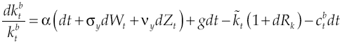
It will be assumed that there is a cost for credit¹, so now capital k~t chased by paying a cost δ > 0 whose dynamics are:

[17]

where dR_k measures capital yield available in financial system, δ is the average yield expected, σ_δ represents yield volatility, v_δ is a leap in the average yield expected, dXt is another Wiener process defined in a fixed space of probability that complies with augmented filtration (Ω, F, (F_t)_t≥0, ℙ), with an independent temporary increases, zero average and variance equal to the temporary increase, meanwhile dQt is a new Poisson process characterizing the dynamics leap into the capital yield, with an intensity θ_δ so that:

[18]

[19]

[20]

Process dX_t and dQt are uncorrelated, initial number of leaps in capital yield is Q₀ = 0. Consequently, lender agent will get at the end of every period k~t+ dRk k~t = k~t (1+dRk) obviously borrower agent will pay the same amount. With this, budget constraints of each agent are modified and when equation [17] is substitute into [21] and [22] for lender and borrower, respectively, we have:

[21]

[22]

where dU_t and dM_t are Poisson diffusion processes that results from the modification of capital accumulation equation, for lenders and borrowers respectively, and also all the processes involved are not correlated each other. Now, making decisions by representative agents consider restrictions [21] and [22] and information available at t = 0 determined by F0=k0 ,Z0 ,k~0  ,Q0 ,M0  simultaneously.

Macroeconomic equilibrium

To determine macroeconomic equilibrium, it is needed to establish the balance of the household sector, which under the established conditions is the same for borrowers and lenders, and is ruled by the same scheme that previous section provided. Macroeconomic equilibrium now relies on individual equilibrium of both types of producers.

Lender agent equilibrium

The lender agent makes its decisions based on the conditions set by equation [2] subject to constraint [21], therefore the corresponding optimal trajectories are:

[23]

[24]

[25]

Borrower agent equilibrium

The borrower agent makes decisions based on the conditions set by equation [2] subject to constraint [22], therefore the corresponding optimal trajectories are:

[26]

[27]

[28]

Economic growth rate

The economic growth rate, when there is a capital market, relies on the average growth of both productive sectors lender and borrower, so that by considering equations [21], [22], [25] and [28] the deterministic component of growth is:

[29]

Equivalently,

[30]

The growth rate of an economy without financial system is exactly equal to that one with an efficient financial system; the preceding is verified because equations [12] and [30] are equal. This means that economy grows at the same rate when financial system allows the reallocation of capital so that all producers carry out their production processes. At first sight it may seem that the effect of the financial system on growth is zero, however this is not so because it depends on the level of capital cost at the financial system, a scenario that will be discussed in the next section. If deterministic component of growth is given by [30], then stochastic variability of growth rate is equal to conditions [13] and [14].

Credit constraints and inefficiency of financial system

In previous section it was shown that economic growth rate of an economy with an efficient financial system is equal to that of a non-financial system economy. This is true as long as reallocating unused capital in the economy be the only function of financial system, nevertheless, if financial system is expanding its scope and is looking for a variety of activities with the aim of obtaining a profit derivative from resources management deposited in it, then it can generate inefficiencies within that market, which would increase cost of capital. This same consequence resulting from credit constraints, i.e., limiting the use of capital or little capital available for productive credit generates high capital costs.

And it is precisely a high cost that generates negative impacts on growth. Consider budget constraints set to borrower agent [21] and assume that cost of capital, determined by equation [17], is so high that causes the constraint to be zero or negative. In other words, to achieve

if this is so, then there are two possible scenarios, namely: first one is when a producer wants to maintain a fixed level of consumption and thus a high cost in capital leads to sacrificing its debt, and the second one is to keep up debt payments by sacrificing consumption. Under any scenario, producers has an incentive to not carrying out his economic activities since would not be optimal to do it because they will not obtain the necessary gains to survive, which implies in a fall of economic growth rate being that because borrower sector will not produce. If so, economic growth rate would be:

[31]

Obviously, the economic growth rate established in [31] is less than that set out in [30], i.e. α+avyθy-ρ/Nl<α+αvyθy-ρ. It is in this case when financial system has a negative effect on growth. Accordingly, an excessive increase incapital cost caused by credit constraints or inefficiencies in the financial system generates disincentives in the productive sector and thus creates a fall in economic growth rate, as well as unemployment of production factors. The increase can be measured by the average expected cost δ, by the volatile component σ_δ, as well as by unexpected leaps measured by v_δ.

Optimal behavior of the tax cost of capital

As already discussed, government intervention occurs by a tax on capital yield when capital cost is too high. However, taxation must be paid by someone and as only the financial system or lender agents are subject to such a phenomenon, two possible scenarios can come about. The first occurs when financial system seeks to obtain profits due to discretional allocations of capital in his possession, causing two types of capital yields: the one that financial system obtains and the one lender receives from financial system, obviously with an existing gap between both, being lower the yield that lender receives. If so, then the financial system must undertake the cost of tax.

The second scenario is precisely originated when lender agent asks for a high payment due to the loan of his remaining capital; under this scenario tax must be borne by him. Nonetheless, tax cannot reach such a high level which causes capital accumulation in lender sector to be zero or negative, as if so growth rate of that sector would be negatively affected. Consequently, it met that:

[40]

If you are replacing into above equation equilibrium conditions [3], [23], [24], and if is considered deterministic and stochastic components of processes that represent both capital yield and product, and then clears for capital yield tax, then it is obtained:

[41]

Given that in equation [38] the parameter ω is unknown, then the level of tax cannot be determined and the lower limit depends on capital yield. However, considering conditions [37] and [41] it can be characterized an optimum range, per unit of time, within tax on capital can be placed, namely:

[42]

When government intervention is necessary thru a financial system regulation, the tax on capital yield should follow the optimal behavior determined by the equation above; this way government ensures the participation of both lender and borrower sectors in economic activities and thus will avoid the fall of economic growth rate.

Growth rate with financial regulation

So far it has shown how government intervenes in the economy if financial system has inefficiencies. With such an intervention capital accumulation equations from lenders and borrowers producers are modified, so that now:

[43]

[44]

Thus, deterministic economic growth rate is:

[45]

where, according to restriction [39], public components of the average in government spending and capital yield tax will be canceled. This implies that government regulation only generates the economy to develop at the growth rate set out in section “Aggregate behavior”. Even more, it can be verified clearly that government intervention only corrects the distortions caused by inefficiencies of financial system on the economy. Finally, variability in economic growth rate would be:

[46]

Similarly, condition [39] reverses the effects of regulation.

Data and methodology

The dataset collected for the analysis includes information belonging to 40 developed and emerging countries and referring to the period ranging from 2000 Government financial regulation and to 2013. The choice of the countries sampled in the study answers the need of giving a faithful and unbiased representation of real economy and is carried out by building a balanced set of an equal number of developed and developing countries².

Annual growth rate of each considered country in the analysis is estimated and regressed on a subset of variables in order to evaluate whether a relation-ship between financial sector and economic growth can be found and how such correlation is affected by government regulation and fiscal policy. The period considered for the analysis is rather emblematic in this sense, so that it studies the change in global economy in the aftermath of the financial crisis of 2008 and highlights the difference in magnitude and significancy of coefficients estimated with particular focus on the pre-crisis period, commonly assumed to be particularly importance for the level of wellbeing, development and innovation.

To assess the interaction between financial system, growth rate and government intervention (through policies and regulations), a set of initial regressions is run to first identify the relationship each variable singularly has with the growth rate. This technique enables to evaluate which variables can be relevant for the analysis and how their coefficient changes as we allow them to vary once additional variables are included. The ultimate goal is to demonstrate how the underlying relationship can be affected by potential inefficiencies in the financial sector (proxied by financial variables), the level of existing regulation and government intervention (proxied by the Measures of Economic Freedom) and the impact on real economy by highlighting the trade-off between investments in the productive sector or in financial markets.

The study will thus divide the data collected in two periods based on whether they belong to pre-crisis (2000-2007) or post-crisis (2007-2013) period and differentiate the countries sampled in developed and developing. Any change in the sign, magnitude and significancy of coefficients between the two periods suggests that the aforementioned relationship is in fact sensitive to economy-wide and cross-country factors. Following is the list of variables employed for the model and the theoretical underpinning to justify their inclusion in the analysis.

Variables description

A list of the variables employed, their definition, the unit of measure, the source from which data were collected and the expected sign of their relation with the dependent variable is reported in Table 1.

Table 1: Variable description 

Source: Own alaboration

Methodology

The research computes the estimates by using Ordinary Least Squares (OLS) up-to-date techniques. Notwithstanding the frequent substitution for proxy variables, the choice of regressors does not completely remove any bias caused by endogeneity problems and the small time period and sample size coupled with large fluctuations and external shocks generate dispersed values inside the range, increasing the overall variability, due also to the high heterogeneity of the countries analyzed, and reducing the predictability of the estimates.

The omitted variables bias, instead, is not found to be of main concern. Moreover, proxy variables can only be at most an approximation of the underlying relationship and arbitrary variables such as Fiscal Freedom, Gross Capital Formation, Financial Freedom can only to a certain extent represent the economic fundamentals they are underpinning. Several variables have not been included in the empirical analysis due to the unavailability or reliability of data and, when available, usually present particularly low t-statistics.

However, the results obtained prove the theoretical model and show a reasonably high level of significancy and consistency in the estimates. It would, then, be recommendable to extend the analysis to a larger set of countries, reduce the dispersion in the errors and contain the missing data problem. The estimated equation for the analysis is [45] described in section 4, while the empirical part related to government regulation refers to equation [60].

Results in the pre-crisis model

Table 2 refers to the analysis carried out for developed and developing countries focusing on the period ranging from 2000 to 2007. Column I shows separately the rate of growth for developed and developing countries and highlights the higher rate of growth for the latter (5.3%), suggesting that the first category has already reached its steady state equilibrium growth rate, while emerging economies are still catching up with rich countries due to their recent development. A regression using a constant instead of the dummy Developed = 0 was run but was not included here for sake of brevity and displays the same results found before.

Table 2: Pre-crisis model estimations 

Note: bold: significancy < 0.01; underline: significancy < 0.05; cursive: significancy < 0.10.

Source: Own elaboration.

In Column II, it is directly tested the effect of Lending Rate (or equivalently for the cost of capital) and the coefficient estimated proves the negative relationship with growth rate at all levels of significancy, as demonstrated previously in the theory. Alternatively, the extent and depth of financial system (Domestic Credit to Private Sector) are found to be positively correlated with the dependent variable, even though only mildly (Column III). In order to assess the relationship between the stock market size and growth, Column IV and V compare the results found using respectively S&P Global Equity Indexes and the logarithm of market capitalization (Stkcapital). An initial regression was run using the level values instead of the logarithm of Stkcapital, resulting in an extremely low coefficient and low significancy and t-statistics due to the magnitude and broad dispersion of the values considered. Using log-values, instead, we obtain significant estimates at all levels, much as in Column V. Column VI summarizes the main results obtained related to evidence of the importance of the financial markets in determining growth and in particular the impact of potential imperfections and inefficiencies on the economy. Moreover, it highlights how the previous relationships hold once we include more variables, as shown by the high significancy of the estimates and the value of the goodness-of-fit (36%).

The second part of Table 2 analyzes the role of government in boosting growth. In particular, there is compelling evidence that lower Central Government Debt (Column VIII), higher Fiscal Freedom (Column IX) and a highly but not excessive regulatory system (Column VII) are beneficial to the economy, as shown in the theoretical part. It goes without saying that coercion and full control on economic freedom, property ownership, the rights to freely move labor, capital and goods beyond necessary are harmful for the economy and do not grant respect and protection on individual liberty and constraints resources allocation, undermining growth paths.

The full model in Table 3 indicates interactions between financial and public sector and the ultimate link with GDP growth. Some of the relationship found earlier do not hold once we account for a wider array of variables; however, the predictive power of the test is enhanced (R2 equal to 48%) and GDPgro is indeed determined by the market capitalization of shares, the extent and depth of financial markets, the size of Central Government Debt and the overall level of Fiscal Freedom in the economy.

Table 3: Pre-crisis period-Full model 

Note: bold: significancy < 0.01; underline: significancy <0.05; cursive: significancy < 0.10. Source: Own elaboration.

Source: Onw elaboration

Results in the post-crisis model

Most of the relationships found earlier in the paper do not hold in the post-crisis period. Single regressions were run to test for the significancy of Lending Rate, Financial Freedom and Domestic Credit to Private Sector; however, they were not found to be relevant and for sake of brevity were not reported here. The lower values of the goodness-of-fit is mainly due to the high variability characterizing the period, in particular the recession due to the financial crisis of 2007-8 and followed by a recovery of the worldwide economy in the second half of the period. Negative values found for the first part of the interval were offset by the positive amount of the last years, eliminating any possible results that could have been achieved. Moreover, high dispersion of the values assumed and the greater variance in the errors contributed to the poor fit of the test.

However, market capitalization of shares, the size of the financial market and Fiscal Freedom are confirmed to be positively related to GDPgro, although only singularly and not jointly. Surprisingly, inflation was found to be significant and positively correlated with GDPgro, which is at odds with economic theory. In conclusion, for developed and developing countries the rate of GDPgro shows that both categories of countries were negatively affected by the financial crisis and presented lower rates of growth.

Table 4: Pre-crisis model estimations 

Note: bold: significancy < 0.01; underline: significancy < 0.05; cursive: significancy < 0.10.

Source: Own elaboration.

Results in full-fledged model

The full-period model is built by introducing interaction variables and using the binary variable Crisis to compare the coefficients of the two periods. The results found match the previous analysis: the rate of growth is higher for developing countries than for developed ones and this holds both in the pre-crisis and post-crisis period; the overall rate of growth is significantly higher in the first period than in the second; the binary variable presents an exceptionally high coefficient, leading to the conclusion that it is indeed responsible for the previous result; moreover, its effect is significant both when used singularly and when interacting with the remaining variables; the negative impact of cost of capital is evident only in the pre-crisis and not in the post-crisis period, while the relationship ruling SP_equity, Stkcapital and GDPgro maintains its significancy (although SP_equity in the second period exhibits a puzzling negative sign, not confirmed by the similar variable Stkcapital).

Table 5: Full-fledged model estimations 

Note: bold: significancy < 0.01; underline: significancy <0.05; cursive: significancy < 0.10. Source: Own elaboration.

Trade-off (full period)

To conclude the empirical part, it was fundamental to include a section showing the comparison of financial markets and the productive sector and their effect on growth within the full period of time. This was accomplished by running a regression differentiating the countries sampled in developed and developing (using the once again significant binary variable Developed); however, the results employ data belonging to the full period, underlining the general validity of the findings in Table 6.

Table 6: Trade-off (full period) estimations 

Note: bold: significancy < 0.01; underline: significancy <0.05; cursive: significancy < 0.10.

Source: Own elaboration.

Gross Capital Formation (proxy for the return on the productive sector) and SP_equity (representing the return on investments in the financial system) contribute to determine the overall level of growth; however, the goodness-of-fit in Column I is more than twice the size of the second test, pointing at the chief role of this sector in global economy.