Productivity Shocks in the Short and Long-Run: An Intertemporal Model and Estimation

 

Choques de la productividad en el corto y largo plazo: un modelo y estimación intertemporales

 

Pu Chen*, Gang Gong**, Armon Rezai***, Willi Semmler****

 

* University of Bielefeld, <pchen@uni-bielefeld.de>

** Tsinghua University, <gongg@nankai.edu.cn>

*** Schwartz Center of Economic Policy Analysis, New School, <armon.rezai@gmail.com>

**** Schwartz Center of Economic Policy Analysis, New School, and Center for Empirical Macroeconomics, <semmlerw@newschool.edu>

 

Received December 2007.
Accepted February 2008.

 

Abstract

The nexus between productivity growth and unemployment has been studied in various ways for a long time. In this paper we present a new one, which is to disaggregate data on productivity growth into its short and long-run component. First, we discuss some important contributions in the literature studying the relationship between productivity growth and unemployment both in the short-run and long-run perspective. Second, to study the effects of productivity growth on unemployment more rigorously we formulate a dynamic general equilibrium model in which the agents optimize their decision in two stages. The dynamic general equilibrium model predicts a positive effect of productivity on unemployment in the short-run and a negative unemployment effect in the long. Third, we explore the effect of productivity growth on unemployment empirically. Using Maximum Likelihood Estimation (MLE) and Structural Vector Autoregression (SVAR), we are able to find the theoretical hypotheses in a diverse set of empirical data.

Key words: RBC models, unemployment, productivity growth.

Clasificación JEL: E24, E30, O40

 

Resumen

El nexo entre crecimiento de la productividad y el desempleo se ha estudiado de varias maneras durante mucho tiempo. En este trabajo presentamos una más, en la que se desagregan datos sobre el crecimiento de la productividad en sus componentes de corto y largo plazos. Primero, discutimos algunas contribuciones importantes en la literatura que estudian la relación entre el crecimiento de la productividad y el desempleo desde una perspectiva de corto y largo plazo. Segundo, para estudiar más rigurosamente los efectos del crecimiento de la productividad sobre el desempleo formulamos un modelo de equilibrio general dinámico en el cual los agentes optimizan sus decisiones en dos etapas. El modelo de equilibrio general dinámico predice un efecto positivo de la productividad sobre el desempleo en el corto plazo y un efecto negativo en el largo. Tercero, exploramos empíricamente el efecto del crecimiento de la productividad sobre el desempleo. Para ello usamos la Estimación de Máxima Probabilidad (MLE por sus siglás en inglés) y la Autoregresión de Vectores Estructurales (SVAR) con el fin de encontrar las hipótesis teoricas en un conjunto diverso de datos empíricos.

Palabras clave: modelos RBC, desempleo, crecimiento de la productividad.

 

Introduction

The relationship between productivity growth and unemployment has been debated ever since the classical economists. Already Ricardo asked whether technical progress is a virtue or vice. Most economists maintain that long-run technical progress and growth have led to a rising standard of living in advanced countries. Others claim that technical progress and productivity growth may have contributed to unemployment. This is often stated with respect to European economies with their high rate of unemployment since the end of the 1980's.

The nexus of productivity and employment is also important for the study of Okun's Law. If employment is correlated with output, but does not reveal a one-to-one relationship as Okun (1962) states it, the relationship may change over time, due to changing growth rates of productivity.

Thus, the study of the impact of productivity on employment becomes a relevant issue. After Okun's study was published in 1962, many authors have been involved in this discussion of the relationship of productivity and employment either from the short-run or long-run perspective. Particularly relevant authors are Tobin (1993), Kaldor (1985), Solow (1997) and Rowthorn (1999). We will discuss their contribution, in section 2 of the paper. We also want to mention that ever since the Real Business Cycle (RBC) theorists have postulated technology shocks as driving force of business cycles, an extensive controversy over the relationship of employment and productivity growth has started. In RBC models technology shocks, output and employment (measured as hours worked) are predicted to be positively correlated. This claim has been made the focus of numerous econometric studies. Employing the Blanchard and Quah (1989) research agenda by using Vector Autoregression (VAR) estimates, studies by Gali (1999), Gali and Rabanal (2005), Francis and Ramey (2004) and Basu et al. (2006) find a negative correlation of employment and productivity growth, once account is taken of both demand and supply shocks affecting output.

While most of the econometric work has studied the effects of productivity growth on employment (hours worked), using a VAR methodology, we want to shift the emphasis to the nexus of productivity growth and unemployment in our paper. Although unemployment rates may be impacted by population growth, demographic shifts, changing labor market participation rates of certain parts of the population and so on, one might presume that the demand side of labor, the offered employment by firms, is the most essential factor for driving the unemployment rate.

In this paper we frame the discussion of the relationship between productivity and unemployment into a dynamic general equilibrium model, in which the representative firm and representative household optimize their decisions. The short-run and the long-run relations between the productivity and the unemployment are the result of the specific dynamic property of the model due to demand shocks and technology shocks.

To quantify these short-run and long-run relations we apply two econometric methods. First, we employ a Maximum Likelihood (ML) method to estimate the short-run and the long-run effect simultaneously. Second, we use a structural VAR with long-run restrictions similar to the work starting with Blanchard and Quah (1989). Here we presume that in the long-run non-technology shocks cannot exert a permanent effect on productivity.

 

Stylized facts

Using the data set by Francis and Ramey (2004), which among other data contains time series for productivity growth and employment from 1889 to 2002, one can observe the following stylized facts. Over the last 100 years, total employment grew tremendously and was in 2002 6.5 times higher than in 1889. This corresponds to an annual growth rate of 1.6% in employment. At the same time, however, labor productivity increased by 2.4% p.a. and was in 2002 13.5 times higher than it was in 1889. Real output expanded in this period with an annual growth rate of 3.4% and was in 2002 67 times its 1889 value. This shows that the United States (US) economy has undergone significant changes in the last 100 and something years. However, the picture is even more complicated as the dynamics are not as smooth and constant as one might hope. Not only has there been tremendous structural change (change of employment from agriculture to manufacturing and subsequently to the service sector), but there are also shifts in time trends. As a result the economy's characteristics have clearly changed after 1950.

Especially when looking at productivity growth, one can observe that changes have become less volatile and more persistent. The correlation between various parameters varies also with the time span considered. Nonetheless, Uhlig (2006) points out that all of these coefficients are positive and that, therefore, technical progress and growth in Gross Domestic Product (GDP) are certainly not harming employment and over most periods net employment is created.¹

Uhlig (2006) used the data set developed by Francis and Ramey (2004). Using data supplied by the Bureau of Labor Statistics (bls), one can expand the set by the unemployment series for this period. This enables one to show that this assessment of Uhlig and others has to be treated with caution. Separating the long and short-run effects by taking 10 years averages and the actual deviation thereof, one can relate short and long-run productivity growth and unemployment.² A closer examination of the data, then, reveals clear differences for the long and short-run and, as mentioned above, for the periods before and after World War II (WWII) (i.e. 1890-1930 and 1945-2002).

Uhlig's conclusions that productivity growth does not harm employment and that the structural change after WWII is not significant for this assessment can be proven to be incorrect. In the short-run productivity and unemployment can be positively correlated. Yet, for the different periods, the long and short-run relationship between productivity growth and unemployment can take on slightly different slopes. Specifically, the short-run productivity growth and unemployment are positively correlated after the Second World War, while the result is ambiguous in the period 1890 to 1930.

Due to those structural changes in the relationship between unemployment and productivity growth, we limit our investigation to the post-WWII period. For this time span data availability and data quality is also much better and this allows us to use quarterly data. This data is, again, taken from the bls. Specifically, it includes the unemployment rate and productivity in non-farming business from 1959Q1 to 2005Q4. Figures 1 display the relationship between these two series. As for the previous data, one can observe that unemployment and short and long-run productivity growth are correlated positively and negatively, respectively. Note that the averaging period that has been used here is 12 years.

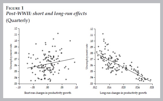
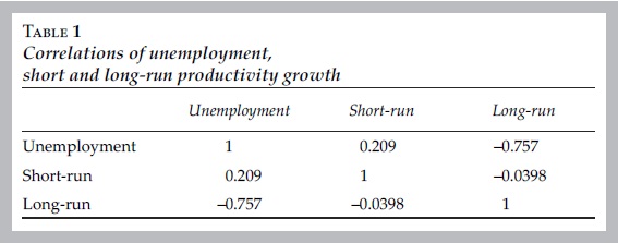
These trends can also be observed in table 1 which depicts the correlations between the unemployment rate and short and long-run productivity growth. While short-run productivity growth and unemployment are weakly positively correlated, long-run productivity growth is strongly negatively correlated with unemployment. One can also see that the two productivity series are virtually not correlated at all. This is important for section 4 where they are assumed to be independent of each other.

One relevant factor that may influence the relation between the technology growth and the unemployment is demand. To eliminate this influence we use in this study the purified technology growth data given in Basu et al. (2006) and study the relation between the technology growth and unemployment. A scatter plot of the unemployment rate on the purified technology growth shows a slightly positive correlation among them.

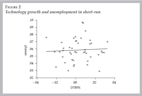
A sample regression of unempl_t on DTBFK_t leads to the following results.

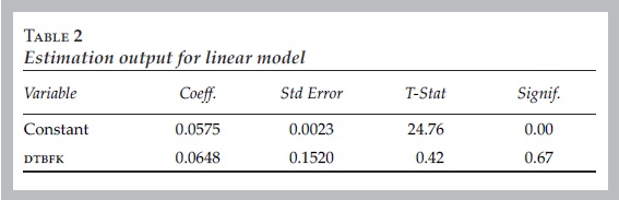
The positive coefficient before DTBFK is insignificant, implying that there is no linear relation between DTBFK_t and unempl_t.

To explore the possible long-run relation among the technology growth and the unemployment we generate scatter plots of their moving averages at various bandwidths (see figure 3).

It can be clearly seen that while the short-run correlation is slightly positive, the long-run correlation at a period length of 10 years becomes negative.

Given these results one is tempted to conclude that productivity shocks (here measured in growth rates of productivity) are likely to increase unemployment in the short term and to reduce unemployment in the long term, as some of the classical literature and also some of the critics of the RBC literature focus on.

 

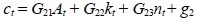
A model of the short and long-run effects of productivity shocks

In order to explain the above mentioned short and long-run effects of technology shocks we suggest a macroeconomic model that follows closely established standards in the literature. It allows for both productivity shocks as well as demand shocks. This will help us to explain the puzzle that in the short-run a technology shock may have a different effect on unemployment than in the long-run.

Our model is based on an intertemporal decision model where the household determines its consumption and leisure pattern with respect to a budget constraint and an accumulated capital stock. The economy is subject to a continuous stream of technology shocks. In our variant there is a search and matching in the labor market which will allow labor market transactions to take place out of equilibrium. If supply and demand for labor do not match, there are constraints for households and households are subsequently allowed to re-optimize. As money is not included in this model, price dynamic is neglected and wages represent real wage developments.

To take a shortcut, we can presume, as the Dynamic General equilibrium (DGE) model does, that the economy is characterized by a representative household and a representative firm. Agents enter market exchanges in three markets: the product, the labor and the capital market. The household owns all factors of production and sells factor services to the firm and buys its products for consumption or accumulation of the capital stock. The product market is assumed to be imperfectly competitive, with the firm facing a perceived demand curve and a sticky price.

Unlike the standard DGE model with competitive markets, the market in this model will be re-opened at the beginning of each period t, necessary to ensure adjustment in response to a non-cleared labor market after the first round of a matching process. The non-clearing of the market in the matching process is caused by wage stickiness as the sequence of wages {w_t}^∞_t=0 is contracted and preset at t = 0 and will not be allowed to change even if the market does not clear. The decision process, therefore, has two stages: in a first step, households determine their consumption and labor supply pattern, in a second step, in case labor demand does match labor supply, households re-optimize their consumption plans following the realized transactions on the factor market.

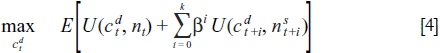
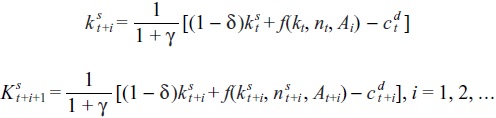
In the first step, at period t = 0, the household expects a series of technology shocks {E_t A_t+1}^∞_i=0and real wages and interest rates {E_tw_t+i, E_tr_t+i}^∞_i=0. The decision problem of the household is then to choose a sequence of planned consumption and labor effort {c^d_t+1, n^s_t+i}^∞_i=0 such that:

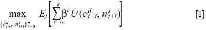
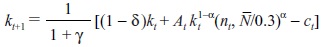
subject to c^d_t+i + i^d_t+i = r_t+i k^s_t+1+ w_t+i n^s_t+i + π_t+i

where superscripts d and s stand for demand and supply, β designates the intertemporal preference rate, δ the depreciation rate, π firms' profits and Y stands for the stationarity parameter. Using standard dynamic programming techniques, this optimal planning problem can be solved to yield the solution sequence {c^d_t+1, n^s_t+i}^∞_i=0; however, from each sequence only the first tupel (c^d_t, n^s_t) is actually carried out.

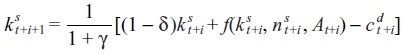
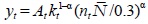
In the period t = 0, the firm decides upon its inputs (k^d_t, n^d_t) given expected demand for its products Ey_t related to its perceived demand curve. Standard (one-period) profit maximization yields the factor demand functions:

As the capital market is supposed to be perfectly competitive, the rental rate of capital, r_t, adjusts in each period such as to clear the market: k_t = k^s_t= k^d_t. On the labor market, however, the fixed wage contract does usually not allow to clear the market.³

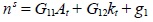
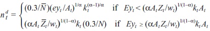
We presume nominal wage rigidity in the first period, such that actual employment does not correspond to labor supply for that period. In order to determine the matching process and actual transactions on the labor market, a matching function employing a rule for employment has to be defined.⁴ For the short side rule there is indeed a long tradition of macroeconomic modeling with specification of the non-clearing labor markets, see, for instance, Benassy (1995, 2002) and Malinvaud (1994). We want to allow labor transactions off the labor demand schedule. So the matching rule we want to use here can be described as:

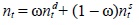
where ω measures the degree to which employment is determined by labor demand and (1 - Co) by labor supply. In this context then, n_t is the actual employment.⁵

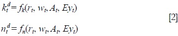
Once the factor inputs have been determined through this matching process [3], defining the employment n_t, the firm proceeds with deciding its output level. Note that the firm is constrained not only by a potentially non-cleared labor market but also by the prospects of a non-cleared product market demand, Ey_t (recall that prices are fixed). Hence the firm will select the optimal capital stock⁶ to optimize the following program:

where , is the realization of Ey_t in period t, yielding the output supply function y^s_t = f(k_t, n_t, A_t).

Yet, the main issue is, once employment and output have been determined, the household needs to re-optimize triggered by the difference between actual and planned employment levels, resulting from the above matching process [3]. Given the realized factor, transactions (k_t, n_t) the new optimal planning program is:

subject to

which can be used to derive the consumption demand based on realized transactions in the factor markets and the realization of the technology shock in period t.

Next, we need to add certain specifications regarding the preference function, the technology shock and the stationarity of the time series data the model may generate.

The household's instantaneous utility function over consumption, c, and leisure, l = 1 - n is:

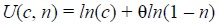
with θ the elasticity between consumption and leisure to be estimated with the data. Moreover, technological shocks are supposed to follow and AR(1) process:

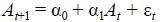
where: ε_t ~ N(0, σ²_ε)

The stationarity parameter, y, can be recovered by calculating the trend growth rate of output. Finally, employment, n_t, is based on (normalized) hours worked (sample mean ). Further the specification of the model can be summarized as follows:⁷

• The evolution of the —stationarized— capital stock.

• The technological evolution.

• The production function.

• Labor supply.

• Labor demand.

• Actual employment.

• Consumption decision.

• Expected production.

The essentials of our model are as follows. Households' demand for goods may be constrained by the firms' actual demand for labor. This way households also constrain the product market in buying less consumption goods than firms would like to be bought. The non-cleared labor market is derived from a multiple stage decision process of households facing constraints in the labor market, but firms are likely to be also constrained, namely constrained in the product market. Here is where the role of demand comes relevant. This additional component of our model gives rise to a further interaction of the labor market and the product market constraints, allowing for non-cleared markets. For further details see Gong and Semmler (2006, 2007).

Overall, however, if firms face constraints on the product market due to insufficient demand, this may explain the technology puzzle, namely that positive technology shocks may have only a weak effect on employment in the short-run —a phenomenon inconsistent with DGE models, where technology shocks and employment are predicted to be positively correlated—. The household's constraints on the labor market spills over to the product market and the firm' constraints on the product market generates employment constraints. One might predict that such a model matches better time series data of advanced economies such as the us and the Euro-area (see Ernst et al., 2006).

If the economy works as above sketched, there is also an important role for aggregate demand. In the standard DGE model there are only technology shocks. They are the driving force of business cycles. Technology shocks are measured by the Solow residual. The Solow residual is computed on the basis of observed output, capital and employment, and it is presumed that all factors are fully utilized. There are several reasons to distrust the standard Solow residual as a measure of technology shock. First, Mankiw (1989) and Summers (1986) have argued that such a measure often leads to excessive volatility in productivity and even the possibility of technological regress, both of which seem to be empirically implausible. Second, it has been shown that the Solow residual can be expressed by some exogenous variables, for example demand shocks arising from military spending (Hall, 1988) and changed monetary aggregates (Evans, 1992), which are unlikely to be related to factor productivity. Third, the standard Solow residual can be contaminated if the cyclical variations in factor utilization are significant.

Considering that the Solow residual cannot be used as a measure of technology shock, since it may embody non-technology shocks researchers have now developed different methods to measure technology shocks correctly. There are basically three strategies. The first strategy is to use an observed indicator to proxy for unobserved utilization. A typical example is to employ electricity use as a proxy for capacity utilization (see Burnside, Eichenbaum and Rebelo, 1996). Another strategy is to construct an economic model so that one could compute the factor utilization from the observed variables (see Basu and Kimball, 1997 and Basu et al, 2006). A third strategy uses an appropriate restriction in a VAR estimate to identify a technology shock (see Gali, 1999 and Francis and Ramey, 2004, 2005).

In the standard DGE model the above mentioned authors find that the technology shock in fact is negatively correlated with employment if one measures technology shocks by the corrected Solow residual.⁸ Though the standard DGE model predicts a significantly high positive correlation between technology and employment, most of the recent empirical research demonstrates, at least at business cycle frequency, a negative correlation. As our preliminary empirical evidence of section 2 shows while this seems to hold true in the short-run, the nexus between productivity and employment may be different in the long-run.

One should, then, distinguish the short and long-run effects for both productivity and demand shocks. Traditionally, only technology shocks have been seen to have persistent effects. In terms of the effects on output and employment in this view, demand shocks have only a short-run effect output and employment but not affecting output and employment in the long-run. On the other hand, productivity increases appear to have long-run effects on output. A set up like this is also presumed in recently used VAR tests with supply and demand shocks. Blanchard and Quah (1989) for example, presume that supply shocks (productivity shocks) have permanent effects on output, but not employment. Demand shocks have, due to nominal rigidities, only a temporary effect on both output and employment.⁹

Yet a model as the one introduced above will predict that in the short-run technology shocks may indeed have a negative effect on employment (positive effect on unemployment). This is predicted to occur when demand is constrained through the above described two stage decision making process. The productivity shock, however, may lead to increasing employment (reduction of unemployment) in the long-run and thus there may be a persistent positive productivity effect on employment in the long-run.¹⁰

 

The econometric methods and results

Next, we will employ two econometric methods to estimate the short and long-run effects of productivity growth on unemployment. First, we construct a model with short-run and long-run components to present the shot-run and long-run effect explicitly. Using maximum likelihood method we can estimate both the short-run and long-run-effect as well as the frequency of the long-run. Second, we employ the generally used technique of a structural vector autoregression (SVAR) with the long-run restriction that non-technology shocks can not permanently increase productivity growth.

The data used for these estimations are the purified technology growth and the unemployment rate from 1947 to 1996.

 

A short-run/long-run components model

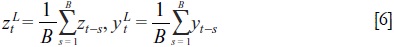
In order to gage the short and long-run effects of productivity growth on unemployment, we assume that both series consist of a short-run and a long-run component:

where z_t is the time series of the unemployment rates i.e. z_t = unempl_t andy_t is the time series of the purified technology growth i.e. y _t = DTBFK_t. Further we assume that the long-run component can be calculated as the moving average of the time series.

Assuming that there exist the following long-run and short-run relations:

where u^L_t ~ N(0, σ²_L) and u^S_t ~ N(0, σ²_S)are independent normal distributed disturbances.

Inserting [7] into [5] we obtain

The density function for the model ([8]) is:

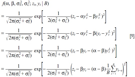
The economic hypotheses under investigation are: α<0 and β>0.

Remarks:

• The long-run short-run model differs from a simple regression model z_t = βy _t in that it adds an "additional" explanatory variable y^f into the regression equation. Hence the goodness of fit will better. It is easy to see that the existence of the estimate, unless y^L_t is colinear with y_t.

• If α = β, the short-run and the long-run relations are identical. The short-run long-run model reduces to the simple regression model.

• If B is given, y^L_t can be calculated from the data and the short-run and long-run model is equivalent to a model with two regressors: y _t and y^L_t.

• If B is unknown, one can calculate the MLE for every possible B and choose B such that the likelihood function is maximized. Since for B = 1 we have the simple regression model and for B = T we have the simple regression model with a constant (if the constant has not been in the specification), therefore we will have an optimal estimate for B.

• The assumption of iid u^S_t and u^L_t is in general too restrictive. Relaxing this assumption is necessary in order to be applicable for more general cases. A direct generalization of this assumption is that the disturbance may follow an AR(1) process: u^S_t+ u^L_t= ρ (u^S_t-1+ u^L_t-1) + ε_t

Applying the maximum estimation method as described above to model [8] extended by remarks 4 and 5, we obtain = 15 and the estimates summarized in the following table (with p as an autoregressive term).

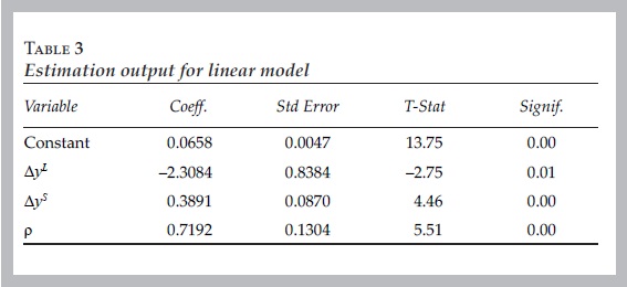
It shows that all of the included variables are highly significant. An increase in long-run 1% productivity growth over a period of 15 years appears to translate in a twice as high reduction of unemployment rate. The effect of short-run productivity growth appears to have a slightly positive effect on unemployment. These results confirm the previous preliminary examination in section 2. In the next section these results are analyzed in the SVAR framework in order to gain deeper insight in the relationship between productivity and unemployment.

 

VAR with long-run restrictions

Another way to gage the effects of productivity growth on unemployment is to use the VAR technique. Following the methodology by Gali (1999), we assume that there are technology and non-technology shocks. The assumption that non-technology shocks do not affect productivity growth is, then, used as a long-run restriction.¹¹ The model is similar to Gali's benchmark model, except we replace his measure of employment with the unemployment rate in order to be able to study effects of technology shocks —taken to mean random technology changes— on unemployment. Our approach is different from that of Blanchard and Quah (1989) who assumed supply disturbances do not affect unemployment in the long-run.

To study the effect of technology shocks, we use a structural VAR with long-run restrictions. We presume that in the long-run non-technology shocks cannot exert a permanent effect on productivity growth. If we go by Okun's law, then this long-run effect on output should also translate into a long-run effect on unemployment (see Khemraj et al., 2006), although the Okun coefficient might be diminishing over time. However, we do not impose this restriction. The long-run restriction of a typical VAR is written in vector moving average form as given in the following equations:

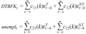
ε^T_t and ε^NT_t are the technology and the non-technology shocks, respectively. If productivity (growth) is unaffected by non-technology shocks in the longrun, it must be that the cumulative effect of such shocks must be equal to zero. That is Σ^∞_k=0c₁₂(k) = 0. Using this restriction we are able to identify the structural VAR and study the effects of technology and non-technology shocks on unemployment.

The likelihood ratio test suggests a lag length of 2 for the reduced form VAR, also the Akaike, the Bayesian, and the Hannan-Quinn information criteria confirm this lag length.

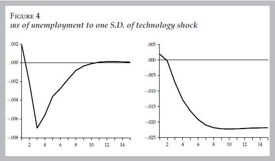
Running a VAR with the above described restrictions, one can compute the Impulse Response Functions (IRFS) using structural decomposition.

Figures 4 depict these functions, the effects of the technology shocks on the unemployment. Unemployment is negatively affected by the technology shocks in the long-run. Comparing this with the results in Basu et al. (2006) and Gali (1991), we confirm largely that the technology shock has a positive employment effect in the long-run.

Conclusion

To study the effects of productivity growth on unemployment we formulate a dynamic general equilibrium model in which the agents optimize their decision in two stages. The dynamic general equilibrium model predicts a positive effect of productivity on unemployment in the short-run and a negative unemployment effect in the long. This reversed effect of productivity growth on unemployment can be identified in a diverse set of empirical data.

To quantify the short-run and long-run effect of the productivity growth on unemployment we apply two econometric methods. In order to concentrate on the effect of technology growth on unemployment we use the purified technology growth data given by Basu et al. (2006). We develop a short-run long-run model to identify the short-run and long relation between the technology growth and unemployment. The maximum likelihood estimation shows that the positive short-run effect and the negative longrun effect are highly significant. The ml estimation also helped us to draw the line between the two time horizons in an optimal way. We also apply the svar with long-run restrictions that the non-technology shocks do not have permanent effect on productivity growth. Our result confirm largely the result in the literature: Basu et al. (2006) uses the methods of SVAR with long-run restrictions and came to the result that the hours worked reacted to the technology shock negatively in the short-run but positively in the long-run. Gali (1999) used SVAR with long restrictions and came to the result that the productivity growth had a negative influence on the employment/hours worked. The initial negative effect is fully reversed over time. We, here, concur as our results show that the technology growth affects unemployment positively in the short-run but negatively in the long-run.

 

References

Basu, S., J.G. Fernald and M.S. Kimball, "Are Technology Improvement Contractionary?", American Economic Review, no. 96, 2006, pp. 1418-1448.         [ Links ]

Basu, S. and M.S. Kimball, "Cyclical Productivity with Unobserved Input Variation", National Bureau of Economic Research (NBER), Working Papers no. 5915, 1997.         [ Links ]

Benassy, J.P., "Money and Wage Contract in an Optimizing Model of the Business Cycle", Journal of Monetary Economics, no. 35, 1995, pp. 303-315.         [ Links ]

----------, The Macroeconomics of Imperfect Competition and Nonclearing Markets, Cambridge, Massachusetts Institute of Technology (MIT) Press, 2002.         [ Links ]

Blanchard, O., "The Role of Shocks and Institutions in the Rise of European Unemployment: The Aggregate Evidence", in W Semmler (ed.), Monetary Policy and Unemployment. The US, Euro-area, and Japan. Volume in Honor of James Tobin, Routledge International Studies in Money and Banking, 2005.         [ Links ]

Blanchard, O. and D. Quah, "The Dynamic Effects of Aggregate Demand and Supply Disturbances", American Economic Review, no. 79, 1989, pp. 655-673.         [ Links ]

Burnside, C., M. Eichenbaum and S.T. Rebelo, "Sectoral Solow Residual", European Economic Review, no. 40, 1996, pp. 861-869.         [ Links ]

Ernst, E., G. Gong, W Semmler and L. Bukeviciute, "Quantifying the Impact of Structural Reforms", European Central Bank, Working Paper Series no. 666, 2006.         [ Links ]

Evans, C., "Productivity Shock and Real Business Cycles", Journal of Monetary Economics, no. 29, 1992, pp. 191-208.         [ Links ]

Francis, N. and V.A. Ramey, "The source of Historical Economic Fluctuations: An Analysis Using Long-run Restrictions", NBER, Working Papers no. 10631, 2004.         [ Links ]

----------, "Is the Technology-driven Real Business Cycle Hypothesis Dead? Shocks and Aggregate Fluctuations Revisited", Journal of Monetary Economics, no. 52, 2005, pp. 1379-1399.         [ Links ]

Gali, J., "Technology, Employment, and the Business Cycle: Do Technology Shocks Explain Aggregate Fluctuations?", American Economic Review, no. 89, 1999, pp. 249-271.         [ Links ]

Gali, J. and P. Rabanal, "Technology Shocks and Aggregate Fluctuations: How Well does the RBC Model fit Postwar U.S. Data?", International Monetary Fund (IMF), Working Papers no. 04/234, 2005.         [ Links ]

Gong, G. and W Semmler, Stochastic Dynamic Macroeconomics: Theory and Empirical Evidence, United Kingdom, Oxford University Press, 2006.         [ Links ]

----------, "Business Cycles, Wage Stickiness and Nonclearing Labor Market", Center for Empirical Macroeconomics, Working Paper, 2007.         [ Links ]

Hall, R.E., "The Relation between Price and Marginal Cost in U.S. Industry", Journal of Political Economy, no. 96, 1988, pp. 921-947.         [ Links ]

Kaldor, N., "A Model of Economic Growth", Economic Journal, no. 67, 1957, pp. 591-624.         [ Links ]

----------, Economics without Equilibrium (The Arthur M. Okun Memorial Lectures), M.E. Sharpe, 1985.         [ Links ]

Khemraj, T., J. Madrick and W Semmler, "Okun's Law and Jobless Growth", Schwartz Center for Economic Policy Analysis, Policy Note no. 3, 2006.         [ Links ]

Malinvaud, E., Diagnosing Unemployment, Cambridge, Cambridge University Press, 1994.         [ Links ]

Mankiw, N.G., "Real Business Cycles: A New Keynesian Perspective", Journal of Economic Perspectives, no. 3, 1989, pp. 79-90.         [ Links ]

Okun, A., "Potential gnp: Its Measurement and Significance", Proceedings of the Business and Economic Statistics Section, American Statistical Association, 1962.         [ Links ]

Rowthorn, R., "Unemployment, Wage Bargaining and Capital-labour Substitution", Cambridge Journal of Economics, no. 23(4), 1999, pp. 413-425.         [ Links ]

Semmler, W, W Zhang and A. Greiner, "Monetary and Fiscal Policy in the Euro-area, Macro Modelling, Learning and Empirics", Amsterdam, Elsevier, 2005.         [ Links ]

Solow, R., Learning from "Learning by Doing": Lessons for Economic Growth, Stanford, Stanford University Press, 1997.         [ Links ]

Summers, L.H., "Some Skeptical Observations on Real Business Cycles Theory", Federal Reserve Bank of Minneapolis Quarterly Review, no. 10, 1986, pp. 23-27.         [ Links ]

Tobin, J., "Price Flexibility and Output Stability: An Old Keynesian View", Journal of Economic Perspectives, no. 7(1), 1993, pp. 45-65.         [ Links ]

Uhlig, H., Discussion of "The Source of Historical Economic Fluctuations: An Analysis using Long-run Restrictions" by N. Francis and V.A. Ramey, Sonderfoerderungsbereich 649, Discussion Paper no. 2006-042, 2006.         [ Links ]

 

Notas

We gratefully acknowledge the valuable contributions of Tarron Khemraj in preparation of this paper and two anonymous referees.

¹ Of course, there are distributional aspects of the effects of productivity on employment. Productivity and output growth might increase inequality. Economic growth might not arrive at low levels of income. Uhlig (2006) also hints at those distributional aspects of the productivity and employment nexus.

² Note that we consider moving averages as preferable over HP-filtering since it leaves the time series relatively unaltered.

³ This may nevertheless happen if either the representative firm has perfect foresight on the sequence of technology shocks or the wage contract is done in the form of a contingency plan. Both will be excluded here; see Gong and Semmler (2007) on a discussion on this latter point. In an extension of our model we presume that the wage is partially adjusted to some optimal wage, co*, but it is still very sticky, see Gong and Semmler (2007).

⁴ In disequilibrium literature the short side of the market is supposed to determine the outcome, formalized by the minimization rule: n_t = min(n^d_t, n^s_t ). However, such an assumption may be too restrictive, as employment may need time to adjust from one period to the other.

⁵ Note that we presume that there may be differential impacts of the labor supply or labor demand on the actual employment. So the matching outcome is not necessarily determined by a Nash bargaining process.

⁶ Notice that capital markets clear instantaneously and capital can be adjusted at no cost following an unfavorable realization of the demand shock.

⁷ For farther details, see Gong and Semmler (2006).

⁸ See also Gong and Semmler (2006, chapters 5 and 9) and Basu et al. (2006).

⁹ This position is also replicated in the study of monetary policy analysis, where it is usually assumed that monetary policy shocks only have temporary effects. However, following Blanchard (2005), Semmler, Zhang and Greiner (2005, chapter 6) show that monetary policy affects persistently, both, the real interest rate as well as the real activity and employment.

¹⁰ We want to note, however, that in this context then demand may or may not have effects on unemployment in the long-run, but it may have a persistent effect on productivity in the long-run. This may be pursued further in a framework suggested by Tobin (1993). We do not pursue this line of research here, due to our emphasis on productivity and unemployment.

¹¹ Generally, we could, however, presume that non-technology shocks, along the line of Kaldor (1957), have some effect on productivity but this will be captured by the productivity component.