


 nueva página del texto (beta)
 Inglés (pdf)
 Artículo en XML
 Referencias del artículo
 Enviar artículo por email
 Citado por SciELO
  Similares en
SciELO
Similares en
SciELO 
 Permalink
1. Introduction
Many astrophysical issues, particularly those involving star structure and galactic dynamics, benefit from the use of isothermal models (Binney & Tremaine 1987; Chandrasekhar 1939). In terms of stellar structure and evolution theory, isothermal self-gravitating spheres may be used to calculate the behaviour of physical variables.
There are a lot of studies concerning the isothermal spheres in the framework of Newtonian mechanics (nonrelativistic) (Milgrom 1984; Liu 1996; Natarajan & Lynden-Bell 1997; Roxburgh & Stockman 1999; Hunter 2001; Raga et al. 2013). Several works have conducted numerical investigations on relativistic isothermal spheres within the framework of general relativity theory. Chavanis (2002) explored the structure and stability of isothermal gas spheres using a linear equation of state in the context of general relativity. Sharma (1990) used the Pade approximation technique to provide straightforward and accessible approximate analytical solutions to the TOV equation of hydrostatic equilibrium, and his results indicate that general relativity isothermal arrangements have a limited extent. Saad (2017) proposed a novel approximate analytical solution to the TOV equation using a combination of the Euler-Abel transformation and the Pade approximation. Besides the numerical and analytical solutions of similar nonlinear differential equations similar to TOV equations, artificial intelligence approaches presented reliable results in many problems arising in astrophysics. In this context, Morawski & Bejger (2020) proposed a unique method based on ANN algorithms for reconstructing the neutron star equation of state from the observed mass-radius relationship. Nouh et al. (2020) presented a neural network-based computational approach for solving fractional Lane-Emden differential equation problems. Azzam et al. (2021) used an artificial neural network (ANN) approach and simulate the conformable fractional isothermal gas spheres and compared them with the results of the analytical solution deduced using the Taylor series. Abdel-Salam et al. (2021) presented the neural network (NN) mathematical model and developed a neural network approach for simulating the helium burning network using a feed-forward mechanism.
In the present article, we solve TOV equations by the ANN and analytically by an accelerated Taylor series. We employ an ordinary feed-forward neural network to estimate the solution of TOV equations for the ANN simulation, which has been shown to outperform competing computational approaches. A three-layer feedforward neural network is used, which was trained using a back-propagation learning approach based on the gradient descent rule. The following is the paper’s structure: The relativistic isothermal polytrope is discussed in § 2. The analytical solution to the TOV equation is found in § 3. The mathematical modelling of the ANN is covered in § 4. § 5 summarizes the results obtained, and § 6 presents the conclusion.
2. The Relativistic Isothermal Gas Sphere (RIGS)
In the polytropic equation of state (P = Kρ1+1/n, where P is the pressure, ρ is the density, and K is the polytropic constant), the polytropic index n ranges from 0 to ∞. When n approaches or equals ∞, the isothermal equation of state P = Kρ emerges. By combining the isothermal equation of state with the equation of the hydrostatic equilibrium in the frame of the general relativity, the TOV equation of the isothermal gas sphere could be given as (Sharma 1990),
where Mr is the total mass energy or ‘effective mass’ of the star of radius r including its gravitational field is given by
Define the variables, χ, ν, u, and the relativistic parameter s, by
where ρc and Pc are the central density and central pressure of the star respectively, u(x) and ν(x) are the Emden and is the mass functions of radius, and c is the speed of light. Equations (1) and (2) can be transformed into the dimensionless forms in the (x, u) plane as
which satisfy the initial conditions
If the pressure is substantially lower than the energy density at the center of a star (i.e., goes to zero), as in the non-relativistic case, the system of equations (4) and (5) simplifies to the Newtonian isothermal structure equations
One can calculate physical parameters of the stellar models like radius (R), density (ρ), and mass Mr using the following equations
3. Analytical Solution to Equation (4)
Rearrange equations (4) and (5) as
where the initial conditions are
Write the Taylor series for the function u(x) as
at x = 0 the first derivative is given by
and the second derivative is
differentiating another time, we have
when x = 0 we have
the fourth derivative is given by
when x = 0 we have have v0(4) = 0;
the fifth derivative is given by
Substituting x = 0 we
and so on. Now write the first TOV equation of equation (9) as
Differentiating equation (13) for x we have
when x = 0 all terms are equal to zero.
Differentiating equation (14) for x we have
Putting x = 0 we have
Since
this gives
By differentiating equation (15) and putting x = 0 this gives
Following the same procedure mentioned above, we obtained the values of u''', u0(4) , u0(5), ν0(6) , u0(6) and so on. Substituting these values into the Taylor series, equation (10), the Emden function is given by
4. The Ann Algorithm
4.1. Simulation of the RIGS
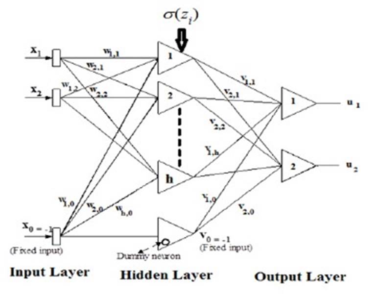
The proposed ANN simulation scheme of the RIGS is plotted in Figure 1. First, we assume ut = (x, p) to be the neural network’s approximate solution to equation (4), which may be expressed as follows (Yadav et al. 2015):
where the first term represents a feed-forward neural network with input vector x and p is the corresponding vector of adjustable weight parameters, and the second term represents the boundary or initial value. The ANN output, N (x, p), is provided by
where zj =
Write the derivative of networks output N for the input vector xj as
and the nth derivative of N, equation (18), is
where
As a result, the proposed solution for the TOV equations is given by
this fulfills the initial conditions as
And
4.2. ANN Gradient Computations and Updating the Parameters
When we examine the solution presented by equations (21), we transform the problem to an unconstrained optimization one, and the error to be minimised is given by (Yadav et al. 2015).
where
To upgrade network parameters, we calculate the NN derivative for both input and the parameters of the network and train the NN for the optimum parameter value. Once the network has been trained, one can optimize the network parameters and compute ut (x, p)ut (x, p) = x2 N(x, p).
The derivative of any of its inputs is analogous to the feed-forward neural network N with one hidden layer, the same weights wij, and thresholds βi, and each weight νi replaced with νi Pi where Pi =
The updating rule of the network parameters will be given as follows
where a, b, c are learning rates, i = 1, 2, ..., n, and j = 1, 2, .., h.
An ANN’s main processing unit is the neuron, which is capable of carrying out local information and processing local memory. The net input (z) of each neuron is calculated by adding the weights it receives to form a weighted sum of such inputs and then adding them with a bias (β). The net input (z) is then processed by an activation function, which is likely to result in neuron output (shown in Figure 1).
4.3. Back-Propagation Learning Algorithm
Back-propagation (BP) is a gradient technique that seeks to minimize the mean square error between the actual and predicted outputs of a feed-forward net. It demands continuously differentiable non-linearity. Figure 2 depicts a flow chart of a back-propagation offline learning method (Leshno et al. 1993). We used a recursive technique that started with the output units and moved back to the first concealed layer. To compare the output uj at the output layer to the desired output tj, an error function of the following kind is used:
For the hidden layer, the error function takes the form:
where δj is the error term in the output layer and wk is the weight between the hidden and output layers. The error is replicated backward from the output layer to the input layer as follows to modify the weight of each connection:

The rate of learning η must be chosen so that it is neither too small, resulting in a slow convergence, nor too large, resulting in misleading results. The momentum term in equation (33) is added with the momentum constant γ to accelerate the convergence of the back-propagation learning algorithm error and to aid in stomping the changes over local increases in the energy function and trying to push the weights to follow the overall downhill direction (Leshno et al. 1993). This term adds a percentage of the most recent weight adjustment to the current weight adjustments. At the start of the training phase, both η and γ terms are allocated and determine the network stability and speed (Elminir et al. 2007; Basheer & Hajmeer 2000; El-Mallawany et al. 2014).
The procedure is repeated for each input pattern until the network output error falls below a preset threshold. The final weights are frozen during the test session and utilized to calculate the precise values of both the density profile and mass-radius relation. To evaluate the training’s success and quality, the error is computed for the entire batch of training patterns using the root-mean-square normalised error, which is defined as:
where P is the number of training patterns, J is the number of output units, tpj is the target output at unit j, and upj is the actual output at the same unit j. Zero error would indicate that all of the ANN’s output patterns completely match the predicted values and that the ANN is completely trained. Internal unit thresholds are also modified by assuming they are connection weights on links derived from an auxiliary constant-valued input.
5. Results and Discussions
5.1. Training Data Preparation
To prepare the data for the ANN simulation of the problem, we elaborated a Mathematica code to derive the Emden and mass functions of the relativistic isothermal gas spheres using the Taylor series. We performed the calculations for the range of the dimensionless parameter x = 0 35; this upper limit of x corresponds to an isothermal sphere on the verge of gravothermal collapse (Antonov 1985). To obtain an accurate result for these analytical physical parameters, we accelerated both the series expansions of the Emden function (u) and the mass function (ν) by the accelerated scheme suggested by Nouh (2004); Saad et al. (2021). The radius, density, and mass of the gas sphere are calculated using equations (8).
We calculated 50 gas models for the range of the relativistic parameter σ = 0 -0.5 with step 0.01. The radius, density, and mass of the star are calculated for the typical neutron star physical parameters: mass M∗ = 1.5M⊙, central density ρc = 5.75 × 10¹⁴ g cm−3, central pressure Pc = 2 × 1033 par, and radius R∗ = 1.4 106 cm. We plotted in Figure 3 the density profiles and the mass-radius relations of the relativistic isothermal gas spheres. Because the effect of the relativistic parameter on the Emden function is smaller than that on the mass function (the relation between the density and the Emden function is given by ρ = ρce−u), we plotted the density profiles for the relativistic parameter values σ = 0.1, 0.2, 0.3, and 0.4 only.
5.2. Network Training
The data calculated in the previous section have been used to train the NN we used to simulate the Emden and mass functions of the relativistic isothermal gas spheres. We trained the ANN that has the architecture previously shown in Figure 1 for such a purpose. The network is composed of three layers which are the input layer, the hidden layer, and the output layer. The input layer has two inputs which symbolize the relativistic parameter (σ) and the ratio (R/R∗), where R∗ is the radius of the typical neutron star which is equal to R∗ = 1.4 106 cm. This ratio takes values from 0 to 1 in steps of 0.02. The output layer has also two outputs which represent the Emden function (density profile) and the mass-radius relation of the relativistic isothermal gas spheres. We checked three configurations for the number of hidden layer neurons by testing 20, 50, and 100 neurons in that layer to find which of them was the best. The data values for the relativistic function (σ) that have been used for the training and testing of the adopted neural network are shown in Table 1.
Table 1 Training and Testing Data for The NN Adopted To Simulate The Emden and Mass Functions of the Relativistic Isothermal Gas Spheres
| Training Data | Testing Data |
|---|---|
| σ | σ |
| 0.01 0.02 0.03 0.05 0.06 | 0.04 0.08 0.12 0.16 0.20 |
| 0.07 0.09 0.010 0.11 0.13 | 0.24 0.28 0.32 0.36 0.40 |
| 0.14 0.15 0.17 0.18 0.19 | |
| 0.21 0.22 0.23 0.25 0.26 | |
| 0.27 0.29 0.30 0.31 0.34 | |
| 0.35 0.37 0.38 0.39 0.41 | |
| 0.42 0.43 0.45 0.46 0.49 | |
| 0.50 |
After checking the three configurations of the hidden layer neurons, we concluded that the best number of those neurons was 50. This number of the hidden layer neurons gave the least RMS error of 0.000156 in almost the same number of training iterations. So, the configuration of the NN adopted to simulate the Emden and mass functions of the relativistic isothermal gas spheres was 2-50-2.
While in the training phase of the NN, we used a value of the momentum (γ = 0.5) and a value for the learning rate (η = 0.03). Those values of γ and η were found to speed up the convergence of the back-propagation training algorithm without exceeding the solution. The convergence and stability behaviors of the input layer weights, bias, and output layer weights (wi, βi, and νi) were studied during the training phase which is shown in Figure 4. The weight values were initialised to random values, which can be seen in such figures, and after a number of iterations, they converged to stable values.

5.3. Comparison with the Analytical Model
After the training phase is completed, we can use the code with its frozen weight values to compute the Emden and mass functions of the RIGS. To compare the analytical models and the ANN ones, we calculated the isothermal gas models for the relativistic parameters shown in Column 2 of Table 1. The results of these comparisons are displayed in Figure 5, which shows the identical overlap between the density profiles and their relevant ANN models. The figures also show the limited discrepancies between the ANN model and their relevant mass-radius relations. In general, we obtained good agreement with a maximum absolute error for the density profiles and mass-radius relations of 1% and 5%, respectively.
Fig. 5 The mass-radius relation and density profile were calculated for the relativistic parameter range σ=0.04, 0,08, 0,12, 0.16, 0.2, 0.24, 0.28, 0.36, and 0.4. The red lines represent the accelerated Taylor series solutions, while the blue lines represent the ANN solutions. The color figure can be viewed online.
According to Nouh et al. (2020), the large discrepancy in the curve of the mass-radius relations can be attributed to numerical instability caused by the mass function’s (ν) acceleration process.
6. Conclusions
In the present paper, the Taylor series and an artificial neural network (ANN) approach were used to solve the relativistic isothermal gas sphere. We wrote a Mathematica code to derive the symbolic expressions for the Emden and the relativistic functions. Then, the radii, densities, and masses of the gas spheres were calculated and the convergence of the analytical models was accelerated using Euler-Abel and Pade transformations. A total sum of 50 analytical gas models was calculated for the range of the relativistic parameter σ =0 0.5 with step 0.01 and compared to the numerical ones which indicated that the maximum relative errors are 1% and 3% for the density profiles and mass-radius relations, respectively.
For the ANN calculations, we developed a C++ code that implemented the feed-forward back-propagation learning scheme. Training and testing of the ANN algorithm were performed for the density profiles and massradius relation of the neutron stars. The efficiency and accuracy of the presented algorithm were evaluated by running it through 10 relativistic isothermal gas models and comparing them to analytical models. The ANN calculations yielded results that were in very good agreement with the analytical results, demonstrating that using the ANN method is effective, accurate, and may outmatch other methods.

