


 text new page (beta)
 English (pdf)
 Article in xml format
 Article references
 Send this article by e-mail
 Cited by SciELO
  Similars in
SciELO
Similars in
SciELO 
 Permalink
1. INTRODUCTION
Since the beginning of the space exploration age, space agencies and, most recently, private companies around the world, have faced the grand problem of vehicle autonomy and the limitations it imposes on a mission’s duration. So far, the most traditional and reliable method of space vehicle’s propulsion is chemical combustion. It requires that part of the overall space and total mass of the vehicle be reserved for the storage of fuel, which in turn will be used for required mission maneuvers. In this manner, it serves as a finite resource and is the main limiting factor of a mission’s length over time. Alternative propulsion systems have long been of interest for agencies and organizations with the purpose of overcoming these problems. A method of propulsion which uses an abundant energy available throughout the whole space in the inner Solar System was conceived in the early 1920s by Soviet scientists Konstantin Tsiolkovsky and Friedrich Zander (McInnes 2004). This energy is called the solar radiation pressure (SRP) and is simply the momentum of the photons emitted by the Sun. In spite of its simple concept, this technology requires a tremendous effort in materials engineering, in order to build structures large enough to absorb sufficient SRP while still having a limited total mass which facilitates its maneuverability (Vulpetti et al. 2015). These structures are denominated solar sails and have increasingly become target of studies (Forward 1990; Angrilli & Bortolami 1990; McInnes 1999; Wie 2007; Guerman et al. 2008; Zeng et al. 2015, 2016; Zhang & Zhou 2017; D’Ambrosio et al. 2019; Meireles 2019) and space missions (Johnson et al. 2011; Fernandez et al. 2014; Palla et al. 2017; Betts et al. 2017a; Viquerat et al. 2015; McNutt et al. 2014; Heiligers et al. 2019; Mori et al. 2020) from the 1990s until today, in order to validate and further explore their propelling concept and promising mission possibilities (McInnes 2003a,b). A special mention must be given to the Japan Aerospace Exploration Agency (JAXA), which has been responsible for significant contributions to the advances and validation of solar sailing and the first ever mission to employ a solar sail: IKAROS (Mori et al. 2010; Tsuda et al. 2011; Mori et al. 2012; Funase et al. 2012; Tsuda et al. 2013). Lastly, the most recent successful mission which employs a solar sail is LightSail-2, from The Planetary Society (Betts et al. 2017b, 2019; Mansell et al. 2020; Spencer et al. 2021). Despite the mission’s successful demonstration of the solar sailing concept, its attitude configuration requires abrupt changes in the spacecraft’s orientation. Considering the difficulty in maneuvering the large surface of the sail with a control system with components sufficiently small to be embarked in the mission, these attitude changes require a greater settling time than ideal for the employed strategy. This causes a SRP acceleration in unwanted directions and jeopardizes the solar sail’s full potential (Plante et al. 2017). Based on this difficulty, this study proposes some alternative approaches, as presented in McInnes (2004), for the use of the solar sail by smoothing the attitude’s rate of change during a maneuver, while still maintaining a similar solar sailing performance.
2. SYSTEM DYNAMICS
The LightSail-2 spacecraft has a total mass m of approximately 5kg and its sail fully deployed has a surface area A of 32m2. Its initial orbit is circular with an altitude of 720km and an inclination of 24◦ (The Planetary Society 2020). Therefore, considering the Earth’s mean radius as 6378km, the initial osculating orbital elements are: semi-major axis of 7098km, eccentricity of 0.0 and inclination of 24◦. The three remaining orbital elements are considered to be zero, due to a lack of further information and their reduced importance for our study.
The dynamical model assumes a 4-body problem, including the Sun, the Earth and the Moon, besides the spacecraft. This means that some of the forces acting on the spacecraft are of gravitational nature, from the Sun, the Earth and the Moon. Nevertheless, a few other perturbation forces were considered in the dynamics. The gravitational potential of a non-spherical Earth was included by using up to the 4th order zonal harmonics perturbation acceleration (Bate et al. 1971). Atmospheric effects were also included to determine the drag forces acting on the spacecraft by taking into account the 1976 U.S. Standard Atmosphere atmospheric model (National Oceanic and Atmospheric Administration (NOAA);National Aeronautics and Space Administration (NASA); United States Air Force (USAF) 1976). Furthermore, a solar radiation pressure (SRP) net force was also considered. It is the propelling force, whose model is presented in details in the next section (Vulpetti et al. 2015). Another widely used model for the SRP force can be found in McInnes (2004). This choice was made based on the existence of legacy codes from previous works developed with the format presented in Vulpetti et al. (2015). Finally, the Earth’s shadow was considered as having a cylinder shaped umbra and no penumbra region to determine a light exposure coefficient for the SRP net force. The orbit was numerically integrated with the use of Cowell’s method (Bate et al. 1971) and a RADAU integrator (Everhart 1985).
LightSail-2 mission’s Attitude Determination and Control System (ADCS) is composed of 5 sun sensors, 4 magnetometers, 2 gyro sensors, 3 torque rods and 1 momentum wheel (Plante et al. 2017). However, this study does not take into consideration the delays from the actuators nor the errors from the sensors. The attitude values used in the orbital simulations are equal to the values proposed by the strategy, in order to compare the difference in their influence in the solar sailing performance.
2.1. Solar Sail Dynamics
To derive the dynamics of a solar sail propelled spacecraft it is convenient to define a Spacecraft Oriented Frame (SOF), as illustrated in Figure 1. The SOF’s X axis points in the radial direction of a heliocentric inertial frame. It has the same direction of the incoming sunlight, which is indicated by the unit vector u. The SOF’s Z axis is defined as having the same direction of the spacecraft’s orbital angular momentum, indicated by the unit vector h. The Y axis is defined in agreement with a coordinate system in dextrorotation. The sail’s orientation is represented by the unit vector n orthogonal to the solar sail surface. Two important angles are consequently defined, the azimuth α and the elevation δ, necessary to resolve n in the SOF. An important consideration is made: the n unit vector exists only in the opposite semi-space of the sunlight beam or, in other words, opposite to the sunlit layer of the solar sail. This limits both the azimuth and elevation angles to the interval [−90,90]◦.

Fig. 1 Spacecraft oriented frame (SOF) referenced at the spacecraft’s barycenter, adapted from Vulpetti et al. (2015).
To determine the thrust T resulting from SRP, as a function of the sail’s orientation, it is furthermore useful to define the lightness vector L, conceived in the SOF as the impulsive acceleration normalized by the Sun’s local gravitational acceleration and defined as
where σ c is a constant referred to as critical loading (equation 2), σ is the sail loading (equation 3), n x is the SOF’s X axis n versor’s component, r spec is the specular reflectance coefficient, r diff is the diffuse reflectance coefficient, χ is the emission/diffusion coefficient (the subscript f refers to the front side of the solar sail), κ is a net thrust dimensionless factor that results from the absorbed and re-emitted power on both sides of the sail (equation 4), and a is the absorptivity coefficient.
The previously mentioned critical loading σ c (equation 2), sail loading σ (equation 3) and net thrust dimensionless factor κ (equation 4), are defined as
where I 1AU = 1366W/m2 is the energy flux emitted by the Sun at 1 Astronomic Unit, the average Sun-Earth distance, equal to 149597870700m, c ≈ 2,9979 × 10⁸ m/s is the speed of light in a vacuum, g 1UA ≈ 5,930 × 10−3 m/s2 is the gravitational acceleration of the Sun at 1 Astronomical Unit, m is the spacecraft’s total mass, A is the solar sail surface area, T is the solar sail’s temperature and is the emittance coefficient as a function of T (again, the subscript f refers to the front side of the sail, while the subscript b refers to the back side). From equation 3 and LightSail-2 mission’s specifications, the sail loading is σ = 156.25g/m2.
Further considerations are made in regard of the optical coefficients absorptivity α, diffuse reflectance r diff and specular reflectance r spec. They are all considered to be a function of the angle of the incident light beam, as portrayed in Figure 2.
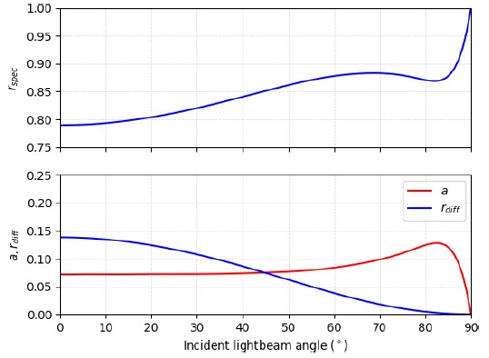
Fig. 2 Absorptivity a, diffuse reflectance r diff and specular reflectance r spec coefficients as a function of the incident light angle for an aluminium sail with a root mean square roughness equal to 20nm (Vulpetti & Scaglione 1999). The color figure can be viewed online.
An incidence angle of 0◦ represents the case where the unit vectors u and n are parallel. Since both the reflectance coefficients are also a function of the sail’s reflective layer roughness, the worst case scenario for the graphs of a value of 20nm root mean square roughness was considered for the simulations.
The Jet Propulsion Laboratory (JPL) published some of its solar sail models coefficients obtained from experimental studies developed in the early 2000’s, which are presented in Table 1 (McInnes 2004). The values of and χ of a square solar sail were used for this study.
3. ATTITUDE STRATEGIES
This section serves the purpose of explaining in details each of the three different strategies, as presented in McInnes (2004) and used to simulate the solar sail’s orientation and their consequences to the spacecraft’s orbital trajectory. The results obtained from the Planetary Society strategy are used as a reference for comparison to the other two strategies analyzed by this study.
3.1. Strategy 1: The Planetary Society
The Planetary Society initial strategy consists of operating the solar sail at an “on-off” regime (Mansell et al. 2020). It consists of maintaining the solar sail at full exposure to the sunlight whenever the spacecraft is traveling away from the Sun. In other words, the unit vector orthogonal to the sail n is parallel to u and, consequently, both the azimuth and elevation angles α and δ are equal to zero. On the other hand, the “off” regime consists of maintaining the solar sail without any exposure to the sunlight whenever the spacecraft is traveling in the direction of the Sun. This means that the unit vectors n and u are orthogonal between themselves and α and/or δ are equal to 90◦. The schematics of this strategy is illustrated in Figure 3.

Fig. 3 LightSail-2 orientation schematics, adapted from Betts et al. (2017b). The color figure can be viewed online.
In order to maximize the thrust component in the SOF XY-plane, δ is always equal to zero. Consequently, only the value of α changes. The first day of simulation (with the purpose of zooming in the X axis) for this strategy is illustrated in Figure 4.

It is possible to observe that two attitude maneuvers are necessary at every orbital revolution.
The first 200 days of the orbital dynamics of this system were simulated using Strategy 1, as well as the spacecraft’s altitude evolution, are presented in Figure 5.
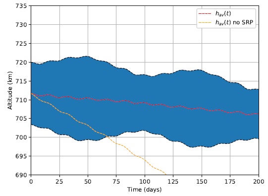
Fig. 5 Spacecraft’s altitude as function of time for Strategy 1. The color figure can be viewed online.
The blue region of the plot is in fact the altitude over time. It is seen as a blur due to the large scale of time covered in the X axis. As expected, it behaves as a sinusoidal wave enveloped by two other curves of the maximum and minimum altitude reached at every revolution, which in turn are seen as the dashed black lines. The dashed red line is a simple average of the envelope curves and is considered to be the average altitude as a function of the simulation instant in days h av(t[days]). It starts at a value of 711.6867km and decreases 5.5204km to 706.1663km after 200 days. The dashed orange line indicates h av(t) for a simulation with disabled solar sailing, meaning a null SRP net force, to demonstrate the importance of solar sailing for maintaining the spacecraft’s average altitude over time. After 200 days, h av(200) = 671.6718km, having lost an extra 34.4945km, or 7.25 times more, of average altitude in comparison with the situation where the solar sailing is active.
Figure 6 presents the actual highest and lowest points of the orbit’s altitude values for the LightSail-2 mission, publicly made available and directly taken from The Planetary Society’s link for the LightSail-2 Mission Control (The Planetary Society 2020). A similar chart can be seen in the same link. There are clear differences from the results seen in Figure 5, despite the fact that the general behavior of these figures are the same. This happens due to the simplified orbital model used in the simulation and to limited access to initial conditions information for the spacecraft. In addition, the model considered overestimates the solar radiation pressure net thrust in comparison to the drag force. Therefore, in order to approximate the simulation results to the LightSail-2’s mission published data, the SRP net thrust had to be scaled down by a factor of 7×10⁻².
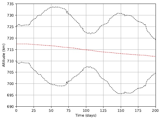
Fig. 6 LightSail-2’s apogee, perigee and average altitude curves as a function of time from LightSail-2 Mission Control (https://www.planetary.org/explore/projects/lightsail-solar-sailing/lightsail-mission-control.html). The color figure can be viewed online.
The initial average altitude of LightSail-2 mission’s at sail’s deployment, on 23 July 2019, is 717.4105km. On 3 February 2020, 200 days after sail deployment, the average altitude is 711.6255km, in contrast to the simulated value of 706.1663km. Although a divergence from the simulated and actual trajectory data is not ideal, it is not a vital requirement for this study that they match in value. As is the case, the main result is a comparison from all the attitude strategies, and since they are all simulated using the same orbital models, the results from Strategy 1 serve mainly as a comparison reference for other strategies.
3.2. Strategy 2: Maximum
Solar radiation pressure propulsion is a specific type of low-thrust. Therefore, the thrust is a function of the spacecraft’s orientation, but for solar sails, its magnitude is also a function of the spacecraft’s position. Therefore, an analysis of its trajectory as a function of its orientation is possible from a traditional approach (Keaton 1986) given this extra constraint |T| = f(n , r), where r is the spacecraft’s position in the heliocentric inertial frame (HIF).
From equation 5, it is known that the specific orbital energy’s rate of change over time is maximized when the net thrust component in the direction of the spacecraft’s velocity vector has its greatest magnitude. This does not necessarily mean (and often it is the case) that the sail and/or the net thrust vector should be pointed in the direction of travel. In equation 5 ṙ is the spacecraft’s velocity vector in the HIF
To determine this optimal strategy, it is necessary to search for the orientation which gives the maximum component of T at the ṙ direction. Considering one point of the simulation at a time, that is to say, having a fixed position r and velocity ṙ, this is a well bound one dimensional convex problem, with α constrained in the interval [−90,90]◦. A simple hill climbing search algorithm is sufficient, and was used in this study to find the solutions. The first day of simulation (again, with the purpose of zooming in the X axis) for this strategy is illustrated in Figure 7.

In contrast to the limited number of attitude maneuvers per orbital revolution from Strategy 1, this approach requires a constant control over the sail’s orientation. Nevertheless, it is possible to observe an interesting characteristic of this strategy’s behavior: the sail completes half a rotation (the azimuth angle α rises from −90◦ to 90◦) for every orbital revolution. This is a crucial information considered in the development of Strategy 3. It is also important to note that, from the definition of unit vector n (it exists in the semi-space opposite to the incoming sunbeam and, put differently, it always points away from the sail’s side not exposed to the sunlight), the transition of value from α = 90◦ to α = −90◦ does not mean a change of 180◦ in the sail’s orientation. In this situation, the unit vector n merely changes its side back to the one in the shadow. Furthermore, for this consideration to work with the simulations in this study, it is necessary for the solar sail to have equally reflective sides.
Figure 8 displays the same quantities presented in Figure 5, but this time, with the employment of Strategy 2.

Fig. 8 Spacecraft’s altitude as function of time for Strategy 2. The color figure can be viewed online.
There is a noticeable quantitative difference between the results of Strategies 1 and 2. The latter presents an average altitude after 200 days of 719.9000km, which is 13.7337km, or 1.94%, higher. But there is also a remarkable contrast between both simulations. While Strategy 1 decreases its average altitude over time, Strategy 2 actually increases its value. Starting from 711.7190km, it gains 8.1810km over the course of 200 days. This result is of great value given the objective of LightSail-2 mission in demonstrating the hidden potential of SRP in maneuvering a spacecraft. The more the solar sail is capable of increasing the average altitude of the spacecraft, the more the concept of solar sailing gains relevance.
3.3. Strategy 3: Constant
From the desire of maintaining a performance in altitude gain close to the one obtained from Strategy 2 while trying to reduce the number of attitude maneuvers, in order to maintain a similarity to LightSail-2 mission’s approach, a third strategy was analyzed. It consists of keeping the sail at a constant rate of change of its azimuth angle
Figure 9 illustrates some examples of the proposed strategy. Every instant of an attitude maneuver is indicated with a red cross in the graph. Once again, only the first day of simulation is presented with the intention of zooming on the X axis values and having a better view for further analysis. The top graph corresponds to an attitude maneuver once every orbital revolution (N rev = 1). The bottom graph corresponds to an attitude maneuver once every five orbital revolutions (N rev = 5).
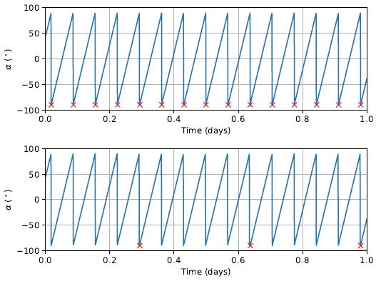
Fig. 9 Azimuth angle α as a function of time for Strategy 3. N rev = 1 for the upper graph. N rev = 5 for the lower graph. The color figure can be viewed online.
Figure 10 presents the azimuth angle rate of change

Fig. 10 Azimuth angle rate of change
From the data presented in Figure 10, it is interesting to observe the general behavior of
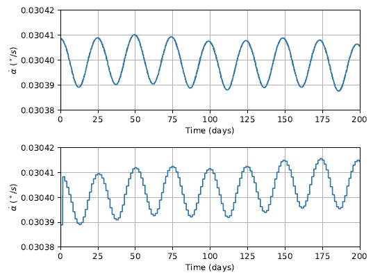
Fig. 11 Azimuth angle rate of change
As ε increases, so does the orbital period. Therefore,
It became interesting to simulate a range of N rev to evaluate for how long the spacecraft can be left without any attitude maneuver and still have a better performance than Strategy 1. The average altitude after 200 days of simulation h av(200) and its gain compared to the initial average altitude h gain (equation 6) are presented in Table 2, as a function of N rev
TABLE 2 EVALUATION OF HAV(200) AS A FUNCTION OF NREV FOR STRATEGY 3
| Nrev | hav(200) (km) | hgain(200) (%) |
| 1 | 711.9803 | +0.0367 |
| 2 | 711.9994 | +0.0394 |
| 3 | 712.0116 | +0.0411 |
| 4 | 712.0119 | +0.0412 |
| 5 | 712.0039 | +0.0400 |
| 10 | 711.8236 | +0.0147 |
| 15 | 711.3687 | -0.0492 |
| 20 | 710.6479 | -0.1505 |
| 25 | 709.6213 | -0.2947 |
| 30 | 708.3483 | -0.4736 |
| 35 | 706.7824 | -0.6936 |
| 40 | 704.9903 | -0.9454 |
| 45 | 702.9148 | -1.2370 |
| 50 | 700.5899 | -1.5637 |
Remarkably, only values of N rev greater than 35 resulted in h av(200) smaller than 706.1663km, obtained by Strategy 1. This means that over 70 times fewer maneuvers could be performed without a loss in the solar sail’s performance in keeping the spacecraft’s average altitude. An unexpected result is having a maximum value for N rev = 4. The expected maximum was found for N rev = 1. Despite this fact, the whole range of N rev from 1 up to 10 presents similar results for h av(200), all of which, as is the case of Strategy 2, show an increase of h av over time. This indicates that other conditions are maybe more significant for this range of values. Results from Table 2 are presented graphically in Figure 12.

Fig. 12 Average altitude after 200 days as a function of N rev for Strategy 3. The color figure can be viewed online.
The blue dashed line at the top is the result obtained from Strategy 2. It can be considered as a maximum, yet unattainable, goal for Strategy 3. On the other hand, the red dashed line at the bottom is the result obtained from Strategy 1. Since it was already implemented in the LightSail-2 mission, it can be considered as a minimum to overcome. For values of N rev smaller than or equal to 35, Strategy 3 proved to be a successful attempt to improve the performance of a solar sail to gain altitude.
4. MISSION PARAMETERS ANALYSIS
In this section, a set of mission parameter values were modified to investigate their general behavior. The use of Strategy 2 is justified as being a theoretical limit to the maneuvering potential of solar sailing. Namely, it is the best case scenario.
An important consideration is made for the average altitude’s change of value over time. It is assumed to have a linear variation along the 200 days simulated. Therefore, it was possible to implement a linear least-squares regression for h
av(t), as indicated in Figure 13 by the yellow dashed line. The slope of these regression lines is henceforth referred to as
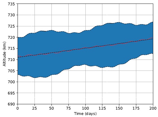
Fig. 13 The spacecraft altitude as a function of time for Strategy 2. The color figure can be viewed online.
As final considerations, after each sweep of the mission parameters, the regression line’s slope values are fitted to a given function, and are presented in the corresponding section.
4.1. Initial Altitude Sweep
An interesting analysis comes from the sweep of the mission’s initial altitude h(0). As indicated by Figure 5, the drag forces are greatly responsible for the spacecraft’s altitude decay. An also known fact is that, as the altitude decreases, the drag forces increase in magnitude. In turn, this would decrease the slope of the regression line. The inverse is also expected to be true. Therefore, a sweep of values in the [690,750]km interval was made (Figure 14). In addition, given the exponential nature of the atmospheric model considered, the data is fitted to the function presented in equation 7
where x is the independent variable from known data, y is the dependent variable for the fitted curve and c n are the function’s parameters.

Fig. 14 Average altitude slope after 200 days as a function of the initial altitude h(0) for Strategy 2. The parameters of equation 7 are also displayed. The color figure can be viewed online.
Figure 14 shows that Strategy 2 can avoid the decay of the spacecraft for initial altitudes close to 700km. Since the atmospheric model only considers that the atmosphere’s density is not null up to an altitude of approximately 865km, and therefore drag forces only exist until this altitude, it is interesting to extend the interval of analysis to verify that greater values of h(0) do not fall near the fitted curve and behave in a different manner, closer to a linear behavior (Figure 15).

4.2. Spacecraft Mass Sweep
A fundamental parameter for solar sailing is the sail loading σ (equation 3). As the spacecraft’s mass m increases, so does σ, and consequently the sail’s capacity to maneuver the spacecraft decreases (equation 1). Given that Strategy 2 was able to increase h av(t) over time, an effort was made to determine how much m could be increased while keeping a constant sail size (and surface area A) and still maintaining a positive slope for the average altitude regression line (Figure 16). Given the nature of equation 1, the data is fitted to the function presented in equation 8
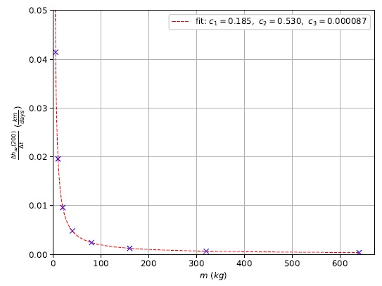
Fig. 16 Average altitude after 200 days as a function of the spacecraft’s mass for Strategy 2. The parameters of equation 8 are also displayed. The color figure can be viewed online.
The figure shows that, even for a massive spacecraft of nearly half a ton, the regression line’s slope still maintains a positive value. Despite being a fitted parameter, the fact that c 3 is greater than zero indicates a limit, given this mission’s initial conditions and the employment of Strategy 2, which would guarantee no decay for the spacecraft’s average altitude. It means that, in theory, any spacecraft can use this technique.
In the search for negative
TABLE 3 CURVE FIT PARAMETERS FOR THE AVERAGE ALTITUDE*
| h(0) | c1 | c2 | c3 |
| 720 | 0.185 | 0.530 | 0.000087 |
| 715 | 0.147 | 0.538 | 0.000099 |
| 710 | 0.107 | 0.526 | 0.000112 |
| 705 | 0.063 | 0.330 | 0.000118 |
| 700 | 0.019 | -3.681 | 0.000104 |
| 695 | -0.035 | 1.671 | 0.000133 |
| 690 | -0.090 | 1.398 | 0.000128 |
* Slope of the regression line after 200 days as a function of the initial altitude h(0) for Strategy 2.

4.3. Orbital Plane Inclination Sweep
Solar sails are an intriguing propelling method with a unique peculiarity. Considering an heliocentric inertial frame, their resulting thrust will always have a radially positive component. As long as a sail is open, it will reflect the incident sunlight, transfer linear momentum to or from the spacecraft to produce a resulting thrust with a positive radial component, whether this is a desired effect or not. The only alternative to avoid the aforementioned limitation is to reduce the sail’s exposed surface area to zero. From a mission control perspective, this would mean increasing either the azimuth angle α or the elevation angle δ to 90◦.
When considering a problem with the objective of increasing the average altitude over time, the desired direction in which the resulting SRP acceleration component needs to be maximized is different for various values of the orbital plane inclination. This results in slightly different desired azimuth angles over the span of an entire orbital revolution. In addition, it would be interesting to investigate different mission scenarios, considering whatever engineering limitations or obligations an organization might have in determining the orbital plane inclination of its mission. Inevitably, the variation of this orbital parameter is another interesting analysis to be made (Figure 18). Given the trigonometric relation of this parameter to the system’s dynamics, the data is fitted to the form presented in equation 9

Fig. 18 Average altitude after 200 days as a function of the orbital plane inclination i for Strategy 2. The parameters of equation 9 are also displayed. The color figure can be viewed online.
As is well known, a smaller exposed surface area results in a lower SRP net thrust. In turn, this means lower specific orbital energy gains or losses and, theoretically, a reduced solar sailing maneuverability. But this fact could be used to the mission advantage. In the situation of higher inclinations, the use of Strategy 2 is specially capable of making the best use of the minimization of losses. In other words, whenever the spacecraft is traveling in the direction of the Sun, the energy losses can be reduced even further, compensating the inferior energy gains. This justifies the increasing average altitude regression line slope, as seen in Figure 18. It also shows that the strategy works for all ranges of inclinations studied [0,90]o but, since
Once again, the initial altitude was changed to lower values, followed by the same curve fit procedures, in the search for a minimum orbital plane inclination where Strategy 2 is capable of maintaining a positive
TABLE 4 CURVE FIT PARAMETERS FOR THE AVERAGE ALTITUDE*
| h(0) | c1 | c2 | c3 | c4 |
| 720 | 0.080 | 0.022 | 8.799 | 0.015 |
| 710 | 0.097 | 0. 022 | 8.672 | -0.009 |
| 700 | 0.118 | 0. 022 | 8.982 | -0.037 |
| 690 | 0.152 | 0. 022 | 7.482 | -0.079 |
| 680 | 0.208 | 0.021 | 4.076 | -0.144 |
| 670 | -0.365 | 0.018 | -9.752 | -0.312 |
| 660 | 2.664 | 0.007 | -132.831 | -2.626 |
* Slope of the regression line after 200 days as a function of the initial altitude h(0) for Strategy 2.
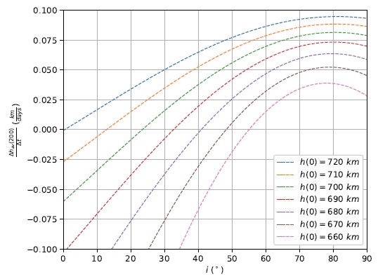
Fig. 19 Curve fit for the average altitude regression line’s slope after 200 days as a function of the orbital plane inclination i for Strategy 2 and different initial altitudes h(0). The color figure can be viewed online.

Fig. 20 Average altitude regression line’s slope after 200 days maximum and null values as a function of the orbital plane inclination i and the initial altitude h(0). The color figure can be viewed online.
Figure 20 also displays a dashed red line that represents the mean value of i for
5. CONCLUSION
This study had the purpose of investigating different attitude strategies for the LightSail-2 mission and how they affect the solar sail’s capacity of maintaining the spacecraft’s altitude over time. Strategy 1 effectively replicated the original approach from the LightSail-2 mission and its implementation served as a base of comparison. Strategy 2, as expected, achieved a maximum performance result, at the cost of constantly maneuvering the sail with small attitude corrections. This strategy made it even possible to increase the spacecraft’s average altitude over time. Strategy 3 presents a simpler alternative to implement a smaller number of attitude maneuvers to keep the solar sail at a desired performance. Its implementation could mean a decrease of more than 70 times the number of attitude maneuvers implemented in LightSail-2’s mission without losing its solar sail’s maneuverability. For cases of up to one maneuver every 10 orbital revolutions, the sail also proved to be able to increase the spacecraft’s average altitude over time.
Making use of Strategy 2’s better performance, the values of the spacecraft’s mass, initial altitude and orbital plane inclination were changed in desired intervals to investigate regions where the sail could still maintain an average altitude gain over time. It was determined that, for the same inclination and for a wide range of spacecraft’s masses of up to half a ton, the initial altitude could be reduced by 20km to a value of 700km. In addition, the sail’s performance could be increased with a raise in the inclination, with a best case scenario for the highest value of 90◦. In turn, with this inclination, the initial altitude could be reduced a further 50km to a value of 650km.
Having examined the final results achieved and given the initial objectives, this study was successful in analyzing alternative attitude strategies able to keep a desired solar sail performance, while still keeping a simple enough implementation for the attitude control system employed in the LightSail-2 mission.

